1. Paper replication

Section 1.1 - Data check

Show code
import pandas as pd
import numpy as np
from pathlib import Path

data_path = Path("data/strategy_returns.xlsx")
xl = pd.ExcelFile(data_path)
print("Sheet names:", xl.sheet_names)
Sheet names: ['XSEC - Carry1m', 'XSEC - Carry1-12', 'TIMING - Carry1m to 0', 'TIMING - Carry1m to mean']
Show code
# Inspect each sheet: columns and first 5 rows
for sheet in xl.sheet_names:
    df = pd.read_excel(xl, sheet_name=sheet, nrows=5)
    print(f"\n=== {sheet} ===")
    print("Columns:", list(df.columns))
    print(df.head())

=== XSEC - Carry1m ===
Columns: ['Dates', 'EQ ', 'FI-LVL', 'FI-SLP', 'FX', 'COM', 'TR', 'CR', 'OC', 'OP']
       Dates  EQ   FI-LVL  FI-SLP  FX  COM  TR  CR  OC  OP
0 1969-12-31  NaN     NaN     NaN NaN  NaN NaN NaN NaN NaN
1 1970-01-30  NaN     NaN     NaN NaN  NaN NaN NaN NaN NaN
2 1970-02-27  NaN     NaN     NaN NaN  NaN NaN NaN NaN NaN
3 1970-03-31  NaN     NaN     NaN NaN  NaN NaN NaN NaN NaN
4 1970-04-30  NaN     NaN     NaN NaN  NaN NaN NaN NaN NaN

=== XSEC - Carry1-12 ===
Columns: ['Dates', 'EQ ', 'FI-LVL', 'FI-SLP', 'FX', 'COM', 'TR', 'CR', 'OC', 'OP']
       Dates  EQ   FI-LVL  FI-SLP  FX  COM  TR  CR  OC  OP
0 1969-12-31  NaN     NaN     NaN NaN  NaN NaN NaN NaN NaN
1 1970-01-30  NaN     NaN     NaN NaN  NaN NaN NaN NaN NaN
2 1970-02-27  NaN     NaN     NaN NaN  NaN NaN NaN NaN NaN
3 1970-03-31  NaN     NaN     NaN NaN  NaN NaN NaN NaN NaN
4 1970-04-30  NaN     NaN     NaN NaN  NaN NaN NaN NaN NaN

=== TIMING - Carry1m to 0 ===
Columns: ['Dates', 'EQ ', 'FI-LVL', 'FI-SLP', 'FX', 'COM', 'TR', 'CR', 'OC', 'OP']
       Dates  EQ   FI-LVL  FI-SLP  FX  COM  TR  CR  OC  OP
0 1969-12-31  NaN     NaN     NaN NaN  NaN NaN NaN NaN NaN
1 1970-01-30  NaN     NaN     NaN NaN  NaN NaN NaN NaN NaN
2 1970-02-27  NaN     NaN     NaN NaN  NaN NaN NaN NaN NaN
3 1970-03-31  NaN     NaN     NaN NaN  NaN NaN NaN NaN NaN
4 1970-04-30  NaN     NaN     NaN NaN  NaN NaN NaN NaN NaN

=== TIMING - Carry1m to mean ===
Columns: ['Dates', 'EQ ', 'FI-LVL', 'FI-SLP', 'FX', 'COM', 'TR', 'CR', 'OC', 'OP']
       Dates  EQ   FI-LVL  FI-SLP  FX  COM  TR  CR  OC  OP
0 1969-12-31  NaN     NaN     NaN NaN  NaN NaN NaN NaN NaN
1 1970-01-30  NaN     NaN     NaN NaN  NaN NaN NaN NaN NaN
2 1970-02-27  NaN     NaN     NaN NaN  NaN NaN NaN NaN NaN
3 1970-03-31  NaN     NaN     NaN NaN  NaN NaN NaN NaN NaN
4 1970-04-30  NaN     NaN     NaN NaN  NaN NaN NaN NaN NaN
Show code
# Load main sheet fully (XSEC - Carry1m is cross-sectional carry with 1-month signal)
df_xsec = pd.read_excel(xl, sheet_name='XSEC - Carry1m', parse_dates=['Dates'])
df_xsec = df_xsec.set_index('Dates')
df_xsec.columns = df_xsec.columns.str.strip()  # Clean column names

# Check data availability per column
print("Data range and count per strategy:")
print(df_xsec.dropna(how='all').describe().loc[['count', 'mean', 'std']])
Data range and count per strategy:
               EQ      FI-LVL     FI-SLP          FX         COM          TR  \
count  295.000000  347.000000  347.00000  347.000000  392.000000  493.000000   
mean     0.797974    0.320929    0.05628    0.441130    0.934718    0.038358   
std      3.025243    2.150447    0.18993    2.252609    5.421549    0.194282   

               CR          OC          OP  
count  476.000000  192.000000  192.000000  
mean     0.020243    5.295643   14.908322  
std      0.150751   49.510091   28.665455  

Section 1.2 - Strategy Returns and Global Carry Factor Construction

Show code
# Asset class strategy returns from XSEC - Carry1m sheet
# Columns: EQ (Equity), FI-LVL (Fixed Income Level), FI-SLP (Fixed Income Slope),
# FX (Currency), COM (Commodity), TR (Treasury), CR (Credit), OC (Option Call?), OP (Option Put?)

# Define core asset classes (mapping to paper: EQ=equity, FI=bonds, FX=currencies, COM=commodities)
# Combine FI-LVL and FI-SLP for bonds; keep others as-is
# We'll also include CR (credit) and OC/OP (options) if meaningful

# For replication, focus on main asset classes: EQ, FX, COM, and FI (combined or separate)
strategy_cols = ['EQ', 'FX', 'COM', 'FI-LVL', 'FI-SLP', 'CR']
strategies = df_xsec[strategy_cols].copy()

# Show first non-null rows
print("First 5 rows with data:")
print(strategies.dropna(how='all').head())
First 5 rows with data:
            EQ  FX  COM  FI-LVL  FI-SLP      CR
Dates                                          
1973-02-28 NaN NaN  NaN     NaN     NaN -0.0772
1973-03-30 NaN NaN  NaN     NaN     NaN -0.0201
1973-04-30 NaN NaN  NaN     NaN     NaN  0.0609
1973-05-31 NaN NaN  NaN     NaN     NaN  0.0267
1973-06-29 NaN NaN  NaN     NaN     NaN -0.0214
Show code
# Construct Global Carry Factor:
# 1. Volatility-scale each strategy to 10% annualized vol using 36-month rolling window
# 2. Equal-weight average across available strategies each month (require at least 2)
# Returns are in percentage points, so 10% target = 10.0 in our units

VOL_TARGET = 10.0  # 10% annualized (in percentage point units)
ROLLING_WINDOW = 36  # months for rolling std

# Calculate rolling annualized volatility for each strategy (in % terms)
rolling_vol = strategies.rolling(window=ROLLING_WINDOW, min_periods=12).std() * np.sqrt(12)

# Volatility-scaled returns: scale to VOL_TARGET using prior month's vol estimate
# Use shift(1) to avoid look-ahead bias
vol_scaled = strategies / rolling_vol.shift(1) * VOL_TARGET

# Equal-weight global carry: average across strategies with at least 2 non-null
global_carry = vol_scaled.mean(axis=1, skipna=True)
# Mask months with fewer than 2 strategies available
strategy_count = vol_scaled.notna().sum(axis=1)
global_carry = global_carry.where(strategy_count >= 2)

# Combine into final DataFrame
all_strategies = strategies.copy()
all_strategies['Global'] = global_carry

print("Global carry factor (vol-scaled EW) - first non-null rows:")
print(all_strategies['Global'].dropna().head())
Global carry factor (vol-scaled EW) - first non-null rows:
Dates
1981-02-27    1.729916
1981-03-31   -3.311699
1981-04-30    0.099063
1981-05-29   -0.046883
1981-06-30    1.797768
Name: Global, dtype: float64

Section 3 - Summary Statistics (Table II Style)

Show code
# Compute summary statistics for each strategy
# Annualized mean, vol, Sharpe, skewness, excess kurtosis
# NOTE: Returns in the data are already in percentage points (e.g., 0.79 = 0.79%)

def compute_summary_stats(returns_series):
    """Compute summary stats for a monthly return series (assuming rf=0).
    Input returns are in percentage points (e.g., 1.0 = 1%)."""
    r = returns_series.dropna()
    n = len(r)
    if n < 12:
        return pd.Series({
            'Ann Mean (%)': np.nan, 'Ann Vol (%)': np.nan, 'Sharpe': np.nan,
            'Skewness': np.nan, 'Excess Kurt': np.nan, 'N': n
        })
    mean_m = r.mean()  # already in % terms
    std_m = r.std()    # already in % terms
    ann_mean = mean_m * 12  # annualized, still in % terms
    ann_vol = std_m * np.sqrt(12)  # annualized, still in % terms
    sharpe = (mean_m / std_m) * np.sqrt(12) if std_m > 0 else np.nan
    skew = r.skew()
    kurt = r.kurtosis()  # pandas kurtosis is excess kurtosis by default
    return pd.Series({
        'Ann Mean (%)': ann_mean,
        'Ann Vol (%)': ann_vol,
        'Sharpe': sharpe,
        'Skewness': skew,
        'Excess Kurt': kurt,
        'N': n
    })

# Apply to all strategies (asset classes + global)
summary_stats = all_strategies.apply(compute_summary_stats)
summary_stats = summary_stats.T
print(summary_stats.round(2))
        Ann Mean (%)  Ann Vol (%)  Sharpe  Skewness  Excess Kurt      N
EQ              9.58        10.48    0.91      0.24         2.19  295.0
FX              5.29         7.80    0.68     -0.68         1.50  347.0
COM            11.22        18.78    0.60     -0.40         1.58  392.0
FI-LVL          3.85         7.45    0.52     -0.43         3.74  347.0
FI-SLP          0.68         0.66    1.03      0.33         1.97  347.0
CR              0.24         0.52    0.47      1.32        15.35  476.0
Global          7.32         5.43    1.35     -0.45         2.00  380.0
Show code
# Final Summary Statistics Table (Table II Style from Koijen et al.)
from tabulate import tabulate
print(tabulate(summary_stats.round(2), headers='keys', tablefmt='simple'))
          Ann Mean (%)    Ann Vol (%)    Sharpe    Skewness    Excess Kurt    N
------  --------------  -------------  --------  ----------  -------------  ---
EQ                9.58          10.48      0.91        0.24           2.19  295
FX                5.29           7.8       0.68       -0.68           1.5   347
COM              11.22          18.78      0.6        -0.4            1.58  392
FI-LVL            3.85           7.45      0.52       -0.43           3.74  347
FI-SLP            0.68           0.66      1.03        0.33           1.97  347
CR                0.24           0.52      0.47        1.32          15.35  476
Global            7.32           5.43      1.35       -0.45           2     380
Show code
# Check exact data range and file used
print("Data file used:", data_path)
print("\nDate range in dataset:")
print(f"  Start: {df_xsec.index.min()}")
print(f"  End:   {df_xsec.index.max()}")
print(f"  Total months: {len(df_xsec)}")

# Check per-strategy date ranges
print("\nPer-strategy date coverage:")
for col in strategy_cols:
    valid = df_xsec[col].dropna()
    if len(valid) > 0:
        print(f"  {col}: {valid.index.min().strftime('%Y-%m')} to {valid.index.max().strftime('%Y-%m')} ({len(valid)} obs)")
Data file used: data/strategy_returns.xlsx

Date range in dataset:
  Start: 1969-12-31 00:00:00
  End:   2012-09-28 00:00:00
  Total months: 514

Per-strategy date coverage:
  EQ: 1988-03 to 2012-09 (295 obs)
  FX: 1983-11 to 2012-09 (347 obs)
  COM: 1980-02 to 2012-09 (392 obs)
  FI-LVL: 1983-11 to 2012-09 (347 obs)
  FI-SLP: 1983-11 to 2012-09 (347 obs)
  CR: 1973-02 to 2012-09 (476 obs)

2. Extending the paper with a bigger dataset

Section 2.1 - Data check

Show code
# Load extended dataset
data_path_ext = Path("data/strategy_returns_-_global.xlsx")
xl_ext = pd.ExcelFile(data_path_ext)
print("Sheet names:", xl_ext.sheet_names)
Sheet names: ['XSEC - Carry1m', 'XSEC - Carry1-12', 'TIMING - Carry1m to 0', 'TIMING - Carry1m to mean']
Show code
# Load main sheet
df_xsec_ext = pd.read_excel(xl_ext, sheet_name='XSEC - Carry1m', parse_dates=['Dates'])
df_xsec_ext = df_xsec_ext.set_index('Dates')
df_xsec_ext.columns = df_xsec_ext.columns.str.strip()

print("Data range and count per strategy:")
print(df_xsec_ext.dropna(how='all').describe().loc[['count', 'mean', 'std']])
Data range and count per strategy:
               EQ      FI-LVL      FI-SLP          FX         COM
count  401.000000  453.000000  453.000000  453.000000  498.000000
mean     0.656740    0.282549    0.046053    0.349864    0.614686
std      2.781576    1.929815    0.169111    2.139907    5.341627

Section 2.2 - Strategy Returns and Global Carry Factor Construction

Show code
# Extended dataset has: EQ, FI-LVL, FI-SLP, FX, COM (no CR, TR, options)
strategy_cols_ext = ['EQ', 'FX', 'COM', 'FI-LVL', 'FI-SLP']
strategies_ext = df_xsec_ext[strategy_cols_ext].copy()

print("first 5 rows with data:")
print(strategies_ext.dropna(how='all').head(5))

print("\nlast 5 rows:")
print(strategies_ext.tail(5))
first 5 rows with data:
            EQ  FX     COM  FI-LVL  FI-SLP
Dates                                     
1980-02-29 NaN NaN  9.5635     NaN     NaN
1980-03-31 NaN NaN -5.9165     NaN     NaN
1980-04-30 NaN NaN -4.9295     NaN     NaN
1980-05-30 NaN NaN -0.8658     NaN     NaN
1980-06-30 NaN NaN  5.4950     NaN     NaN

last 5 rows:
                  EQ        FX       COM    FI-LVL    FI-SLP
Dates                                                       
2021-03-31  2.936968  3.093420 -0.432861 -0.331424 -0.046175
2021-04-30 -0.287421 -0.808833  7.450097  1.555466  0.089690
2021-05-31  1.580722 -0.514537 -0.296396  0.204032 -0.015321
2021-06-30 -1.531709  0.271198  0.547531  0.597813  0.009063
2021-07-30 -3.305316 -0.927804 -1.739345  1.097475 -0.010923
Show code
# Construct Global Carry Factor (same methodology)
VOL_TARGET = 10.0
ROLLING_WINDOW = 36

rolling_vol_ext = strategies_ext.rolling(window=ROLLING_WINDOW, min_periods=12).std() * np.sqrt(12)
vol_scaled_ext = strategies_ext / rolling_vol_ext.shift(1) * VOL_TARGET

global_carry_ext = vol_scaled_ext.mean(axis=1, skipna=True)
strategy_count_ext = vol_scaled_ext.notna().sum(axis=1)
global_carry_ext = global_carry_ext.where(strategy_count_ext >= 2)

all_strategies_ext = strategies_ext.copy()
all_strategies_ext['Global'] = global_carry_ext

print("Global carry factor - first non-null rows:")
print(all_strategies_ext['Global'].dropna().head())
Global carry factor - first non-null rows:
Dates
1984-11-30    3.105087
1984-12-31    2.495541
1985-01-31    1.464067
1985-02-28    0.158625
1985-03-29    2.641604
Name: Global, dtype: float64

Section 2.3 - Summary Statistics (Full Sample)

Show code
# Full sample statistics (1980-2021)
summary_stats_ext = all_strategies_ext.apply(compute_summary_stats)
summary_stats_ext = summary_stats_ext.T

print(tabulate(summary_stats_ext.round(2), headers='keys', tablefmt='simple'))
          Ann Mean (%)    Ann Vol (%)    Sharpe    Skewness    Excess Kurt    N
------  --------------  -------------  --------  ----------  -------------  ---
EQ                7.88           9.64      0.82        0.28           2.64  401
FX                4.2            7.41      0.57       -0.59           1.48  453
COM               7.38          18.5       0.4        -0.4            1.5   498
FI-LVL            3.39           6.69      0.51       -0.43           4.97  453
FI-SLP            0.55           0.59      0.94        0.51           3.16  453
Global            6.52           5.33      1.22       -0.41           1.33  441

Section 2.4 - In-Sample vs Out-of-Sample Comparison

Show code
# Split at paper end date (Sep 2012)
paper_end = '2012-09-30'

# In-sample (up to Sep 2012)
in_sample = all_strategies_ext.loc[:paper_end]
stats_in = in_sample.apply(compute_summary_stats).T

# Out-of-sample (Oct 2012 onwards)
out_sample = all_strategies_ext.loc[paper_end:].iloc[1:]  # exclude Sep 2012
stats_out = out_sample.apply(compute_summary_stats).T

print("In-Sample (up to Sep 2012):")
print(tabulate(stats_in.round(2), headers='keys', tablefmt='simple'))
print("\nOut-of-Sample (Oct 2012 - Jul 2021):")
print(tabulate(stats_out.round(2), headers='keys', tablefmt='simple'))
In-Sample (up to Sep 2012):
          Ann Mean (%)    Ann Vol (%)    Sharpe    Skewness    Excess Kurt    N
------  --------------  -------------  --------  ----------  -------------  ---
EQ                9.58          10.48      0.91        0.24           2.19  295
FX                5.29           7.8       0.68       -0.68           1.5   347
COM              11.22          18.78      0.6        -0.4            1.58  392
FI-LVL            3.85           7.45      0.52       -0.43           3.74  347
FI-SLP            0.68           0.66      1.03        0.33           1.97  347
Global            7.73           5.31      1.46       -0.33           1.24  335

Out-of-Sample (Oct 2012 - Jul 2021):
          Ann Mean (%)    Ann Vol (%)    Sharpe    Skewness    Excess Kurt    N
------  --------------  -------------  --------  ----------  -------------  ---
EQ                3.15           6.64      0.47       -0.37           0.96  105
FX                0.69           5.9       0.12       -0.32           0.57  105
COM              -6.93          16.98     -0.41       -0.64           1.14  105
FI-LVL            1.86           3.06      0.61       -1              4.12  105
FI-SLP            0.14           0.18      0.79       -0.11          -0.16  105
Global            2.64           5.29      0.5        -0.73           1.56  105
Show code
# Side-by-side Sharpe ratio comparison
comparison = pd.DataFrame({
    'In-Sample Sharpe': stats_in['Sharpe'],
    'Out-of-Sample Sharpe': stats_out['Sharpe'],
    'Difference': stats_out['Sharpe'] - stats_in['Sharpe']
})

print(tabulate(comparison.round(2), headers='keys', tablefmt='simple'))
          In-Sample Sharpe    Out-of-Sample Sharpe    Difference
------  ------------------  ----------------------  ------------
EQ                    0.91                    0.47         -0.44
FX                    0.68                    0.12         -0.56
COM                   0.6                    -0.41         -1.01
FI-LVL                0.52                    0.61          0.09
FI-SLP                1.03                    0.79         -0.23
Global                1.46                    0.5          -0.96

Section 2.5 - Strategy Performance Analysis

Show code
import matplotlib.pyplot as plt
from tabulate import tabulate

def analyze_strategy(returns_series, strategy_name, split_date='2012-09-30'):
    """
    Analyze a strategy with IS/OOS split: cumulative performance chart + statistics table.
    
    Parameters:
    - returns_series: pd.Series of monthly returns (in percentage points)
    - strategy_name: str, name for the chart title
    - split_date: str, date to split IS/OOS
    """
    returns = returns_series.dropna()
    
    # Split into IS and OOS
    is_returns = returns.loc[:split_date]
    oos_returns = returns.loc[split_date:].iloc[1:] if split_date in returns.index else returns.loc[split_date:]
    
    # Compute cumulative returns (convert % to decimal for compounding)
    cum_returns = (1 + returns / 100).cumprod()
    
    # Statistics
    def calc_stats(r):
        if len(r) < 12:
            return {'Ann Mean (%)': None, 'Ann Vol (%)': None, 'Sharpe': None, 
                    'Skewness': None, 'Excess Kurt': None, 'N': len(r)}
        ann_mean = r.mean() * 12
        ann_vol = r.std() * np.sqrt(12)
        sharpe = (r.mean() / r.std()) * np.sqrt(12) if r.std() > 0 else None
        return {
            'Ann Mean (%)': round(ann_mean, 2),
            'Ann Vol (%)': round(ann_vol, 2),
            'Sharpe': round(sharpe, 2) if sharpe else None,
            'Skewness': round(r.skew(), 2),
            'Excess Kurt': round(r.kurtosis(), 2),
            'N': len(r)
        }
    
    stats_is = calc_stats(is_returns)
    stats_oos = calc_stats(oos_returns)
    
    # Create figure
    fig, ax = plt.subplots(figsize=(10, 5))
    
    # Plot cumulative returns
    ax.plot(cum_returns.index, cum_returns.values, 'b-', linewidth=1.5)
    
    # Mark IS/OOS split
    split_dt = pd.Timestamp(split_date)
    if split_dt in cum_returns.index or (cum_returns.index[0] < split_dt < cum_returns.index[-1]):
        ax.axvline(x=split_dt, color='red', linestyle='--', linewidth=2, label=f'IS/OOS Split ({split_date[:7]})')
        
        # Shade regions
        ax.axvspan(cum_returns.index[0], split_dt, alpha=0.1, color='green', label='In-Sample')
        ax.axvspan(split_dt, cum_returns.index[-1], alpha=0.1, color='orange', label='Out-of-Sample')
    
    ax.set_title(f'{strategy_name} - Cumulative Performance', fontsize=14, fontweight='bold')
    ax.set_xlabel('Date')
    ax.set_ylabel('Cumulative Return (Growth of $1)')
    ax.legend(loc='upper left')
    ax.grid(True, alpha=0.3)
    
    plt.tight_layout()
    plt.show()
    
    # Print statistics table
    table_data = [
        ['Ann Mean (%)', stats_is['Ann Mean (%)'], stats_oos['Ann Mean (%)']],
        ['Ann Vol (%)', stats_is['Ann Vol (%)'], stats_oos['Ann Vol (%)']],
        ['Sharpe', stats_is['Sharpe'], stats_oos['Sharpe']],
        ['Skewness', stats_is['Skewness'], stats_oos['Skewness']],
        ['Excess Kurt', stats_is['Excess Kurt'], stats_oos['Excess Kurt']],
        ['N (months)', stats_is['N'], stats_oos['N']]
    ]
    
    print(tabulate(table_data, headers=['Metric', 'In-Sample', 'Out-of-Sample'], tablefmt='simple'))
Show code
analyze_strategy(all_strategies_ext['Global'], 'Global Carry Factor')

Metric          In-Sample    Out-of-Sample
------------  -----------  ---------------
Ann Mean (%)         7.73             2.69
Ann Vol (%)          5.31             5.27
Sharpe               1.46             0.51
Skewness            -0.33            -0.74
Excess Kurt          1.24             1.61
N (months)         335              106
Show code
analyze_strategy(all_strategies_ext['EQ'], 'Equity Carry (EQ)')

Metric          In-Sample    Out-of-Sample
------------  -----------  ---------------
Ann Mean (%)         9.58             3.16
Ann Vol (%)         10.48             6.61
Sharpe               0.91             0.48
Skewness             0.24            -0.37
Excess Kurt          2.19             1
N (months)         295              106
Show code
analyze_strategy(all_strategies_ext['FX'], 'Currency Carry (FX)')

Metric          In-Sample    Out-of-Sample
------------  -----------  ---------------
Ann Mean (%)         5.29             0.61
Ann Vol (%)          7.8              5.87
Sharpe               0.68             0.1
Skewness            -0.68            -0.31
Excess Kurt          1.5              0.59
N (months)         347              106
Show code
analyze_strategy(all_strategies_ext['COM'], 'Commodity Carry (COM)')

Metric          In-Sample    Out-of-Sample
------------  -----------  ---------------
Ann Mean (%)        11.22            -6.83
Ann Vol (%)         18.78            16.9
Sharpe               0.6             -0.4
Skewness            -0.4             -0.65
Excess Kurt          1.58             1.18
N (months)         392              106
Show code
analyze_strategy(all_strategies_ext['FI-LVL'], 'Fixed Income Level (FI-LVL)')

Metric          In-Sample    Out-of-Sample
------------  -----------  ---------------
Ann Mean (%)         3.85             1.88
Ann Vol (%)          7.45             3.04
Sharpe               0.52             0.62
Skewness            -0.43            -1.02
Excess Kurt          3.74             4.18
N (months)         347              106
Show code
analyze_strategy(all_strategies_ext['FI-SLP'], 'Fixed Income Slope (FI-SLP)')

Metric          In-Sample    Out-of-Sample
------------  -----------  ---------------
Ann Mean (%)         0.68             0.15
Ann Vol (%)          0.66             0.18
Sharpe               1.03             0.83
Skewness             0.33            -0.12
Excess Kurt          1.97            -0.19
N (months)         347              106

3. Crypto Carry Factor Construction

Show code
import requests
import pandas as pd
import numpy as np
from pathlib import Path
from datetime import datetime
from dateutil.relativedelta import relativedelta
from tqdm import tqdm
import time
import matplotlib.pyplot as plt
from tabulate import tabulate


DATA_DIR = Path("data")

Section 3.1 - Data Source Validation (Proof of Concept)

Show code
SKIP = False  # Set to False to re-fetch data from Binance

import requests
import pandas as pd

BASE_URL = "https://fapi.binance.com"

if SKIP:
    print("Skipping fetch (SKIP=True). Using cached data if available.")
else:
    # --- 1. Liquidity Filtering: Fetch 24hr volume and identify top 5 USDT-margined assets ---
    ticker_resp = requests.get(f"{BASE_URL}/fapi/v1/ticker/24hr")
    ticker_resp.raise_for_status()

    tickers = pd.DataFrame(ticker_resp.json())
    tickers = tickers[tickers['symbol'].str.endswith('USDT')].copy()
    tickers['quoteVolume'] = tickers['quoteVolume'].astype(float)
    top5_symbols = tickers.nlargest(5, 'quoteVolume')['symbol'].tolist()

    print(f"Top 5 liquid USDT-margined perpetuals: {top5_symbols}")

    # --- 2. Data Sampling: Fetch recent funding rates for top 5 assets ---
    funding_records = []
    for symbol in top5_symbols:
        resp = requests.get(f"{BASE_URL}/fapi/v1/fundingRate", params={"symbol": symbol, "limit": 100})
        resp.raise_for_status()
        records = resp.json()
        for r in records:
            r['symbol'] = symbol
        funding_records.extend(records)

    # --- 3. Data Structure Validation: Combine into DataFrame ---
    funding_df = pd.DataFrame(funding_records)
    funding_df['fundingRate'] = funding_df['fundingRate'].astype(float)
    funding_df['fundingTime'] = pd.to_datetime(funding_df['fundingTime'], unit='ms')
    funding_df = funding_df.sort_values(['symbol', 'fundingTime']).reset_index(drop=True)

    # --- 4. Visualization: Display sample and summary ---
    display(funding_df.head(10))

    summary = funding_df.groupby('symbol')['fundingRate'].agg(['mean', 'min', 'max', 'count'])
    summary.columns = ['Mean Rate', 'Min Rate', 'Max Rate', 'N']
    summary['Ann. Carry (%)'] = summary['Mean Rate'] * 3 * 365 * 100  # 3 funding periods/day
    display(summary.round(6))
Top 5 liquid USDT-margined perpetuals: ['BTCUSDT', 'ETHUSDT', 'ALPACAUSDT', 'SOLUSDT', 'ZECUSDT']
symbol fundingTime fundingRate markPrice
0 ALPACAUSDT 2025-06-15 06:00:00.004 0.000013 0.03103576
1 ALPACAUSDT 2025-06-15 07:00:00.000 0.000013 0.03090201
2 ALPACAUSDT 2025-06-15 08:00:00.009 0.000013 0.03033747
3 ALPACAUSDT 2025-06-15 09:00:00.006 0.000013 0.03060094
4 ALPACAUSDT 2025-06-15 10:00:00.003 0.000013 0.03055576
5 ALPACAUSDT 2025-06-15 11:00:00.000 0.000013 0.03069334
6 ALPACAUSDT 2025-06-15 12:00:00.000 0.000013 0.03082270
7 ALPACAUSDT 2025-06-15 13:00:00.001 0.000013 0.03093763
8 ALPACAUSDT 2025-06-15 14:00:00.000 0.000013 0.03050502
9 ALPACAUSDT 2025-06-15 15:00:00.004 0.000013 0.03022682
Mean Rate Min Rate Max Rate N Ann. Carry (%)
symbol
ALPACAUSDT 0.000012 0.000012 0.000012 100 1.368750
BTCUSDT 0.000053 -0.000028 0.000100 100 5.794904
ETHUSDT 0.000043 -0.000032 0.000100 100 4.687235
SOLUSDT 0.000033 -0.000174 0.000100 100 3.609886
ZECUSDT -0.000065 -0.000827 0.000100 100 -7.069703

Section 3.2 - Rolling Universe Validation (Historical Snapshot Test)

Show code
SKIP = False  # Set to False to re-fetch data from Binance

import requests
import pandas as pd
import matplotlib.pyplot as plt
from tqdm import tqdm
from datetime import datetime

BASE_URL = "https://fapi.binance.com"

# --- Configuration: Simulate decision on Jan 1, 2023 using Dec 2022 data ---
SNAPSHOT_MONTH_START = int(datetime(2022, 12, 1).timestamp() * 1000)
SNAPSHOT_MONTH_END = int(datetime(2022, 12, 31, 23, 59, 59).timestamp() * 1000)
MAX_SYMBOLS = 150  # Limit for speed; set higher for full universe

if SKIP:
    print("Skipping fetch (SKIP=True). Using cached data if available.")
else:
    # --- 1. Fetch all USDT-margined perpetual symbols ---
    exchange_info = requests.get(f"{BASE_URL}/fapi/v1/exchangeInfo").json()
    all_symbols = [
        s['symbol'] for s in exchange_info['symbols']
        if s['symbol'].endswith('USDT') and s['contractType'] == 'PERPETUAL'
    ][:MAX_SYMBOLS]

    print(f"Fetching historical data for {len(all_symbols)} symbols...")

    # --- 2. Fetch Dec 2022 monthly kline (volume) and funding rates ---
    def fetch_monthly_volume(symbol):
        """Fetch Dec 2022 monthly kline, return quote volume."""
        try:
            resp = requests.get(f"{BASE_URL}/fapi/v1/klines", params={
                "symbol": symbol, "interval": "1M",
                "startTime": SNAPSHOT_MONTH_START, "endTime": SNAPSHOT_MONTH_END, "limit": 1
            })
            data = resp.json()
            if data and len(data) > 0:
                return float(data[0][7])  # Quote asset volume
        except:
            pass
        return None

    def fetch_monthly_avg_funding(symbol):
        """Fetch Dec 2022 funding rates, return average."""
        try:
            resp = requests.get(f"{BASE_URL}/fapi/v1/fundingRate", params={
                "symbol": symbol,
                "startTime": SNAPSHOT_MONTH_START, "endTime": SNAPSHOT_MONTH_END, "limit": 1000
            })
            data = resp.json()
            if data and len(data) > 0:
                rates = [float(r['fundingRate']) for r in data]
                return sum(rates) / len(rates)
        except:
            pass
        return None

    # Fetch data with progress bar
    results = []
    for sym in tqdm(all_symbols, desc="Fetching Dec 2022 data"):
        vol = fetch_monthly_volume(sym)
        funding = fetch_monthly_avg_funding(sym)
        results.append({"Symbol": sym, "Volume_Dec2022": vol, "Avg_Funding_Dec2022": funding})

    # --- 3. Construct universe DataFrame ---
    universe = pd.DataFrame(results)
    universe = universe.dropna(subset=['Volume_Dec2022'])
    universe = universe[universe['Volume_Dec2022'] > 0]
    universe = universe.sort_values('Volume_Dec2022', ascending=False).reset_index(drop=True)
    universe['Rank'] = universe.index + 1

    print(f"\n{len(universe)} symbols existed with volume in Dec 2022")
Fetching historical data for 150 symbols...
Fetching Dec 2022 data: 100%|██████████| 150/150 [01:44<00:00,  1.44it/s]

133 symbols existed with volume in Dec 2022
Show code
# --- 4. Diagnostics ---
import os
from tabulate import tabulate

os.makedirs("figures", exist_ok=True)

# 4a. Top 10 most liquid coins from Dec 2022 snapshot
display(universe[['Rank', 'Symbol', 'Volume_Dec2022', 'Avg_Funding_Dec2022']].head(10))

# 4b. Volume drop-off curve (helps decide K)
fig, ax = plt.subplots(figsize=(10, 5))
top100 = universe.head(100)
ax.bar(top100['Rank'], top100['Volume_Dec2022'] / 1e9, color='steelblue', alpha=0.7)
ax.set_xlabel('Liquidity Rank')
ax.set_ylabel('Dec 2022 Volume ($ Billions)')
ax.set_title('Volume Drop-off Curve: Top 100 Coins (Dec 2022)')
ax.axvline(x=30, color='red', linestyle='--', linewidth=1.5, label='K=30')
ax.legend()
ax.grid(True, alpha=0.3)
plt.tight_layout()
fig.savefig('figures/universe_volume_dropoff.png', dpi=150, bbox_inches='tight')
plt.show()
print("Saved: figures/universe_volume_dropoff.png")

# 4c. Funding rate spread: Top 5 vs Bottom 5 liquid
top5 = universe.head(5)
bottom5 = universe.tail(5)

spread_data = [
    ['Top 5 Liquid', f"{top5['Avg_Funding_Dec2022'].mean():.6f}"],
    ['Bottom 5 Liquid', f"{bottom5['Avg_Funding_Dec2022'].mean():.6f}"],
    ['Spread', f"{top5['Avg_Funding_Dec2022'].mean() - bottom5['Avg_Funding_Dec2022'].mean():.6f}"]
]
print(tabulate(spread_data, headers=['Group', 'Avg Funding'], tablefmt='simple'))

display(top5[['Symbol', 'Volume_Dec2022', 'Avg_Funding_Dec2022']])
display(bottom5[['Symbol', 'Volume_Dec2022', 'Avg_Funding_Dec2022']])
Rank Symbol Volume_Dec2022 Avg_Funding_Dec2022
0 1 BTCUSDT 1.651735e+11 0.000046
1 2 ETHUSDT 1.503352e+11 0.000047
2 3 DOGEUSDT 2.289587e+10 0.000022
3 4 BNBUSDT 1.885099e+10 -0.000132
4 5 XRPUSDT 1.273611e+10 -0.000048
5 6 LTCUSDT 1.074952e+10 0.000037
6 7 SOLUSDT 9.236063e+09 -0.000322
7 8 AXSUSDT 8.628874e+09 -0.000405
8 9 MASKUSDT 7.826907e+09 -0.000092
9 10 APEUSDT 6.807995e+09 -0.000927

Saved: figures/universe_volume_dropoff.png
Group              Avg Funding
---------------  -------------
Top 5 Liquid          -1.3e-05
Bottom 5 Liquid       -2e-06
Spread                -1.1e-05
Symbol Volume_Dec2022 Avg_Funding_Dec2022
0 BTCUSDT 1.651735e+11 0.000046
1 ETHUSDT 1.503352e+11 0.000047
2 DOGEUSDT 2.289587e+10 0.000022
3 BNBUSDT 1.885099e+10 -0.000132
4 XRPUSDT 1.273611e+10 -0.000048
Symbol Volume_Dec2022 Avg_Funding_Dec2022
128 ARPAUSDT 1.596212e+08 -0.000093
129 IOTXUSDT 1.394512e+08 0.000089
130 1000XECUSDT 1.052628e+08 -0.000018
131 DUSKUSDT 1.019247e+08 0.000062
132 DEFIUSDT 6.424554e+07 -0.000048

Section 3.3 - Crypto Carry Factor Construction (Full Backtest)

Show code
# Fetching full dataset
import os
import requests
import pandas as pd
import numpy as np
from datetime import datetime
from dateutil.relativedelta import relativedelta
from tqdm import tqdm
import time

PANEL_FILE = "data/crypto_factor/crypto_panel.csv"
FACTOR_FILE = "data/crypto_factor/crypto_factor.csv"

# Skip if data already exists
if os.path.exists(PANEL_FILE) and os.path.exists(FACTOR_FILE):
    print(f"Data already exists: {PANEL_FILE}")
    print("Skipping fetch. Delete files to re-fetch.")
else:
    os.makedirs("data/crypto_factor", exist_ok=True)
    
    BASE_URL = "https://fapi.binance.com"
    START_DATE = datetime(2021, 1, 1)
    END_DATE = datetime(2025, 11, 1)
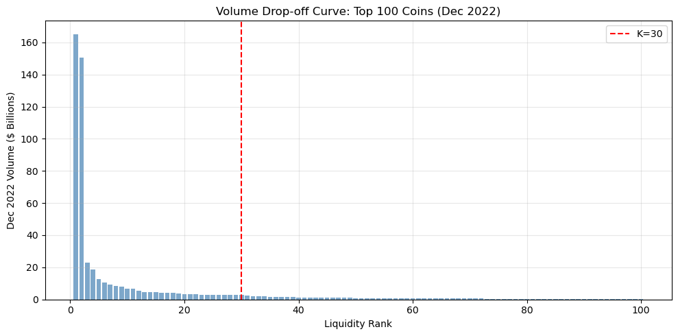
    TOP_K = 30
    API_DELAY = 0.15

    rebal_dates = []
    current = START_DATE
    while current <= END_DATE:
        rebal_dates.append(current)
        current += relativedelta(months=1)

    print(f"Backtest period: {START_DATE.strftime('%Y-%m')} to {END_DATE.strftime('%Y-%m')}")
    print(f"Total months: {len(rebal_dates)}, Universe: Top {TOP_K}")

    def get_all_usdt_perpetuals():
        resp = requests.get(f"{BASE_URL}/fapi/v1/exchangeInfo")
        resp.raise_for_status()
        return [s['symbol'] for s in resp.json()['symbols'] 
                if s['symbol'].endswith('USDT') and s['contractType'] == 'PERPETUAL']

    def get_monthly_volume(symbol, start_ts, end_ts):
        try:
            resp = requests.get(f"{BASE_URL}/fapi/v1/klines", params={
                "symbol": symbol, "interval": "1M", "startTime": start_ts, "endTime": end_ts, "limit": 1})
            data = resp.json()
            return float(data[0][7]) if data else None
        except: return None

    def get_monthly_funding(symbol, start_ts, end_ts):
        try:
            resp = requests.get(f"{BASE_URL}/fapi/v1/fundingRate", params={
                "symbol": symbol, "startTime": start_ts, "endTime": end_ts, "limit": 1000})
            data = resp.json()
            return np.mean([float(r['fundingRate']) for r in data]) if data else None
        except: return None

    def get_monthly_return(symbol, start_ts, end_ts):
        try:
            resp = requests.get(f"{BASE_URL}/fapi/v1/klines", params={
                "symbol": symbol, "interval": "1M", "startTime": start_ts, "endTime": end_ts, "limit": 1})
            data = resp.json()
            if data:
                open_p, close_p = float(data[0][1]), float(data[0][4])
                return (close_p - open_p) / open_p if open_p > 0 else None
        except: pass
        return None

    def month_to_ts(dt):
        return int(dt.timestamp() * 1000)

    def get_month_range(dt):
        start = datetime(dt.year, dt.month, 1)
        end = start + relativedelta(months=1) - relativedelta(seconds=1)
        return month_to_ts(start), month_to_ts(end)

    def compute_factor_return(month_panel):
        if len(month_panel) < 20:
            return None
        sorted_df = month_panel.sort_values('carry_signal', ascending=False)
        long_ret = sorted_df.head(10)['ret_1m'].mean()
        short_ret = sorted_df.tail(10)['ret_1m'].mean()
        return {'date': month_panel['date'].iloc[0], 'long_ret': long_ret, 
                'short_ret': short_ret, 'factor_ret': long_ret - short_ret, 'n_assets': len(month_panel)}

    # Check existing progress
    completed_dates = set()
    if os.path.exists(PANEL_FILE):
        existing = pd.read_csv(PANEL_FILE, parse_dates=['date'])
        completed_dates = set(existing['date'].dt.strftime('%Y-%m-%d'))
        print(f"Resuming: {len(completed_dates)} months done")

    remaining = [d for d in rebal_dates if d.strftime('%Y-%m-%d') not in completed_dates]
    print(f"Remaining: {len(remaining)} months")

    if remaining:
        all_symbols = get_all_usdt_perpetuals()
        print(f"USDT perpetuals: {len(all_symbols)}")

        for i, rebal_date in enumerate(remaining):
            date_str = rebal_date.strftime('%Y-%m-%d')
            print(f"\nProcessing {date_str} ({i+1}/{len(remaining)})")
            
            prior_month = rebal_date - relativedelta(months=1)
            prior_start, prior_end = get_month_range(prior_month)
            
            volumes = {}
            for sym in tqdm(all_symbols, desc="Volume", leave=False):
                vol = get_monthly_volume(sym, prior_start, prior_end)
                if vol and vol > 0: volumes[sym] = vol
                time.sleep(API_DELAY * 0.3)
            
            universe = sorted(volumes.keys(), key=lambda x: volumes[x], reverse=True)[:TOP_K]
            curr_start, curr_end = get_month_range(rebal_date)
            
            records = []
            for sym in tqdm(universe, desc="Signals", leave=False):
                avg_funding = get_monthly_funding(sym, prior_start, prior_end)
                carry_signal = avg_funding * -1 * 3 * 365 if avg_funding else None
                ret_1m = get_monthly_return(sym, curr_start, curr_end)
                records.append({'date': date_str, 'symbol': sym, 'carry_signal': carry_signal, 'ret_1m': ret_1m})
                time.sleep(API_DELAY)
            
            month_panel = pd.DataFrame(records).dropna(subset=['carry_signal', 'ret_1m'])
            month_panel.to_csv(PANEL_FILE, mode='a', header=not os.path.exists(PANEL_FILE), index=False)
            
            factor_row = compute_factor_return(month_panel)
            if factor_row:
                pd.DataFrame([factor_row]).to_csv(FACTOR_FILE, mode='a', header=not os.path.exists(FACTOR_FILE), index=False)
            
            print(f"  ✓ {len(month_panel)} rows, factor_ret={factor_row['factor_ret']*100:.2f}%" if factor_row else "  ✓ Saved")

    print(f"\nComplete: {PANEL_FILE}, {FACTOR_FILE}")
Data already exists: data/crypto_factor/crypto_panel.csv
Skipping fetch. Delete files to re-fetch.
Show code
# Load factor data
from scipy import stats

factor_df = pd.read_csv("data/crypto_factor/crypto_factor.csv", parse_dates=['date'])
returns = factor_df['factor_ret'].dropna()
print(f"Sample: {factor_df['date'].min().strftime('%Y-%m')} to {factor_df['date'].max().strftime('%Y-%m')} ({len(returns)} months)")
Sample: 2021-01 to 2025-11 (59 months)
Show code
# Compute return statistics
mean_ret = returns.mean()
std_ret = returns.std()
skew_ret = returns.skew()
kurt_ret = returns.kurtosis()

ann_mean = mean_ret * 12
ann_vol = std_ret * np.sqrt(12)
sharpe = (mean_ret / std_ret) * np.sqrt(12) if std_ret > 0 else np.nan
jb_stat, jb_pval = stats.jarque_bera(returns)

stats_data = [
    ['Mean (Monthly)', f'{mean_ret*100:.2f}%'],
    ['Mean (Annualized)', f'{ann_mean*100:.2f}%'],
    ['Std Dev (Monthly)', f'{std_ret*100:.2f}%'],
    ['Std Dev (Annualized)', f'{ann_vol*100:.2f}%'],
    ['Skewness', f'{skew_ret:.2f}'],
    ['Excess Kurtosis', f'{kurt_ret:.2f}'],
    ['Sharpe Ratio', f'{sharpe:.2f}'],
    ['Hit Rate', f'{(returns > 0).mean()*100:.1f}%'],
    ['Min Monthly Return', f'{returns.min()*100:.2f}%'],
    ['Max Monthly Return', f'{returns.max()*100:.2f}%'],
    ['Jarque-Bera p-value', f'{jb_pval:.4f}']
]
print(tabulate(stats_data, headers=['Statistic', 'Value'], tablefmt='simple'))
Statistic             Value
--------------------  -------
Mean (Monthly)        0.29%
Mean (Annualized)     3.49%
Std Dev (Monthly)     26.72%
Std Dev (Annualized)  92.56%
Skewness              1.60
Excess Kurtosis       4.42
Sharpe Ratio          0.04
Hit Rate              47.5%
Min Monthly Return    -52.63%
Max Monthly Return    106.29%
Jarque-Bera p-value   0.0000
Show code
# Plot return distribution
import os
os.makedirs("figures", exist_ok=True)

fig, axes = plt.subplots(1, 2, figsize=(14, 5))

# Histogram with normal overlay
ax1 = axes[0]
n, bins, patches = ax1.hist(returns * 100, bins=20, density=True, alpha=0.7, 
                             color='steelblue', edgecolor='black', label='Actual')
x = np.linspace(returns.min() * 100, returns.max() * 100, 100)
normal_pdf = stats.norm.pdf(x, mean_ret * 100, std_ret * 100)
ax1.plot(x, normal_pdf, 'r-', linewidth=2, label=f'Normal(μ={mean_ret*100:.1f}%, σ={std_ret*100:.1f}%)')
ax1.axvline(x=0, color='gray', linestyle='--', alpha=0.5)
ax1.set_xlabel('Monthly Return (%)')
ax1.set_ylabel('Density')
ax1.set_title('Crypto Carry Factor - Return Distribution', fontsize=12, fontweight='bold')
ax1.legend()
ax1.grid(True, alpha=0.3)

# QQ plot
ax2 = axes[1]
stats.probplot(returns, dist="norm", plot=ax2)
ax2.set_title('Q-Q Plot (vs Normal)', fontsize=12, fontweight='bold')
ax2.grid(True, alpha=0.3)

plt.tight_layout()
fig.savefig('figures/return_distribution.png', dpi=150, bbox_inches='tight')
plt.show()
print("Saved: figures/return_distribution.png")

Saved: figures/return_distribution.png

Section 3.4 - Total Return Decomposition (Price + Carry)

The factor return computed above uses only price returns. However, the carry strategy also earns (or pays) funding during the holding period. This section fetches the actual funding rates for each holding month and decomposes total return into:

  • Price Return: (close - open) / open from monthly kline
  • Carry Return: Sum of funding rates during the month (sign-adjusted for position direction)
  • Total Return: Price Return + Carry Return

This helps us understand whether the strategy’s alpha comes from price movements or from persistently earning funding.

Show code
# Fetching current-month funding rates for total return calculation
import os
import requests
import pandas as pd
import numpy as np
from datetime import datetime
from dateutil.relativedelta import relativedelta
from tqdm import tqdm
import time

PANEL_FILE = "data/crypto_factor/crypto_panel.csv"
PANEL_TOTAL_FILE = "data/crypto_factor/crypto_panel_total.csv"
BASE_URL = "https://fapi.binance.com"
API_DELAY = 0.15

if os.path.exists(PANEL_TOTAL_FILE):
    print(f"Data already exists: {PANEL_TOTAL_FILE}")
    print("Skipping fetch. Delete file to re-fetch.")
else:
    panel = pd.read_csv(PANEL_FILE, parse_dates=['date'])
    print(f"Loaded panel: {len(panel)} rows")
    print(f"Date range: {panel['date'].min().strftime('%Y-%m')} to {panel['date'].max().strftime('%Y-%m')}")

    def month_to_ts(dt):
        return int(dt.timestamp() * 1000)

    def get_month_range(dt):
        start = datetime(dt.year, dt.month, 1)
        end = start + relativedelta(months=1) - relativedelta(seconds=1)
        return month_to_ts(start), month_to_ts(end)

    def get_monthly_funding_sum(symbol, start_ts, end_ts):
        try:
            resp = requests.get(f"{BASE_URL}/fapi/v1/fundingRate", params={
                "symbol": symbol, "startTime": start_ts, "endTime": end_ts, "limit": 1000
            })
            data = resp.json()
            if data and len(data) > 0:
                return sum([float(r['fundingRate']) for r in data])
        except:
            pass
        return None

    new_records = []
    for idx, row in tqdm(panel.iterrows(), total=len(panel), desc="Fetching funding"):
        curr_start, curr_end = get_month_range(row['date'])
        funding_sum = get_monthly_funding_sum(row['symbol'], curr_start, curr_end)
        carry_ret_long = -funding_sum if funding_sum is not None else None
        
        new_records.append({
            'date': row['date'].strftime('%Y-%m-%d'),
            'symbol': row['symbol'],
            'carry_signal': row['carry_signal'],
            'ret_1m': row['ret_1m'],
            'carry_ret': carry_ret_long,
            'total_ret': row['ret_1m'] + carry_ret_long if carry_ret_long is not None else None
        })
        time.sleep(API_DELAY)

    pd.DataFrame(new_records).to_csv(PANEL_TOTAL_FILE, index=False)
    print(f"Saved: {PANEL_TOTAL_FILE}")
Data already exists: data/crypto_factor/crypto_panel_total.csv
Skipping fetch. Delete file to re-fetch.
Show code
# Load panel with total returns
panel_total = pd.read_csv("data/crypto_factor/crypto_panel_total.csv", parse_dates=['date'])
panel_clean = panel_total.dropna(subset=['carry_signal', 'ret_1m', 'carry_ret', 'total_ret']).copy()

print(f"Panel: {len(panel_total)} rows, clean: {len(panel_clean)} rows")
Panel: 1770 rows, clean: 1769 rows
Show code
# Define factor return computation
def compute_factor_returns(month_panel, return_col):
    if len(month_panel) < 20:
        return None
    sorted_df = month_panel.sort_values('carry_signal', ascending=False)
    long_ret = sorted_df.head(10)[return_col].mean()
    short_ret = sorted_df.tail(10)[return_col].mean()
    return {'long_ret': long_ret, 'short_ret': short_ret, 'factor_ret': long_ret - short_ret}
Show code
# Compute factor returns for price, carry, and total
factor_records = []
for date, group in panel_clean.groupby('date'):
    price_f = compute_factor_returns(group, 'ret_1m')
    carry_f = compute_factor_returns(group, 'carry_ret')
    total_f = compute_factor_returns(group, 'total_ret')
    
    if price_f and carry_f and total_f:
        factor_records.append({
            'date': date, 'n_assets': len(group),
            'price_long': price_f['long_ret'], 'price_short': price_f['short_ret'], 'price_factor': price_f['factor_ret'],
            'carry_long': carry_f['long_ret'], 'carry_short': carry_f['short_ret'], 'carry_factor': carry_f['factor_ret'],
            'total_long': total_f['long_ret'], 'total_short': total_f['short_ret'], 'total_factor': total_f['factor_ret']
        })

factor_df = pd.DataFrame(factor_records).sort_values('date').reset_index(drop=True)
factor_df['date'] = pd.to_datetime(factor_df['date'])
print(f"Factor returns: {len(factor_df)} months")
Factor returns: 59 months
Show code
# Save decomposed factor returns
factor_df.to_csv("data/crypto_factor/crypto_factor_decomposed.csv", index=False)
print(f"Saved: crypto_factor_decomposed.csv")
Saved: crypto_factor_decomposed.csv
Show code
# Compute summary statistics for each component
def compute_stats(returns):
    mean_m = returns.mean()
    std_m = returns.std()
    return {
        'Ann Mean (%)': mean_m * 12 * 100,
        'Ann Vol (%)': std_m * np.sqrt(12) * 100,
        'Sharpe': (mean_m / std_m) * np.sqrt(12) if std_m > 0 else np.nan,
        'Hit Rate (%)': (returns > 0).mean() * 100
    }

stats_price = compute_stats(factor_df['price_factor'])
stats_carry = compute_stats(factor_df['carry_factor'])
stats_total = compute_stats(factor_df['total_factor'])
Show code
# Print comparison table
comparison_data = []
for metric in ['Ann Mean (%)', 'Ann Vol (%)', 'Sharpe', 'Hit Rate (%)']:
    comparison_data.append([metric, f'{stats_price[metric]:.2f}', f'{stats_carry[metric]:.2f}', f'{stats_total[metric]:.2f}'])
print(tabulate(comparison_data, headers=['Metric', 'Price Only', 'Carry Only', 'Total Return'], tablefmt='simple'))
Metric          Price Only    Carry Only    Total Return
------------  ------------  ------------  --------------
Ann Mean (%)          3.87         25.18           29.05
Ann Vol (%)          92.56          7.09           93.96
Sharpe                0.04          3.55            0.31
Hit Rate (%)         49.15         96.61           55.93
Show code
# Return decomposition insight
price_contrib = factor_df['price_factor'].mean()
carry_contrib = factor_df['carry_factor'].mean()
total_avg = factor_df['total_factor'].mean()

print(f"Decomposition: Price {price_contrib*100:.2f}% + Carry {carry_contrib*100:.2f}% = Total {total_avg*100:.2f}%")
print(f"Dominant source: {'CARRY (funding)' if abs(carry_contrib) > abs(price_contrib) else 'PRICE movements'}")
Decomposition: Price 0.32% + Carry 2.10% = Total 2.42%
Dominant source: CARRY (funding)
Show code
# Compute cumulative returns
cum_price = (1 + factor_df['price_factor']).cumprod()
cum_carry = (1 + factor_df['carry_factor']).cumprod()
cum_total = (1 + factor_df['total_factor']).cumprod()
Show code
# Plot cumulative returns comparison
import os
os.makedirs("figures", exist_ok=True)

fig, ax = plt.subplots(figsize=(12, 5))
ax.plot(factor_df['date'], cum_price, 'b-', linewidth=1.5, label=f'Price Only (SR={stats_price["Sharpe"]:.2f})')
ax.plot(factor_df['date'], cum_carry, 'g-', linewidth=1.5, label=f'Carry Only (SR={stats_carry["Sharpe"]:.2f})')
ax.plot(factor_df['date'], cum_total, 'r-', linewidth=2, label=f'Total Return (SR={stats_total["Sharpe"]:.2f})')
ax.axhline(y=1, color='gray', linestyle='--', alpha=0.5)
ax.set_xlabel('Date')
ax.set_ylabel('Cumulative Return (Growth of $1)')
ax.set_title('Crypto Carry Factor - Cumulative Performance', fontsize=12, fontweight='bold')
ax.legend(loc='upper left')
ax.grid(True, alpha=0.3)
plt.tight_layout()
fig.savefig('figures/return_decomposition.png', dpi=150, bbox_inches='tight')
plt.show()
print("Saved: figures/return_decomposition.png")

Saved: figures/return_decomposition.png
Show code
# Plot monthly return decomposition (stacked)
fig, ax = plt.subplots(figsize=(12, 4))
ax.bar(factor_df['date'], factor_df['price_factor'] * 100, label='Price', alpha=0.7, color='blue')
ax.bar(factor_df['date'], factor_df['carry_factor'] * 100, bottom=factor_df['price_factor'] * 100, 
       label='Carry', alpha=0.7, color='green')
ax.axhline(y=0, color='black', linewidth=0.5)
ax.set_xlabel('Date')
ax.set_ylabel('Monthly Return (%)')
ax.set_title('Monthly Return Decomposition (Price + Carry)', fontsize=12, fontweight='bold')
ax.legend()
ax.grid(True, alpha=0.3)
plt.tight_layout()
plt.show()

Show code
# Rolling 12-month Sharpe comparison
import os
os.makedirs("figures", exist_ok=True)

rolling_window = 12
rolling_sharpe_price = factor_df['price_factor'].rolling(rolling_window).mean() / factor_df['price_factor'].rolling(rolling_window).std() * np.sqrt(12)
rolling_sharpe_carry = factor_df['carry_factor'].rolling(rolling_window).mean() / factor_df['carry_factor'].rolling(rolling_window).std() * np.sqrt(12)
rolling_sharpe_total = factor_df['total_factor'].rolling(rolling_window).mean() / factor_df['total_factor'].rolling(rolling_window).std() * np.sqrt(12)

fig, ax = plt.subplots(figsize=(12, 4))
ax.plot(factor_df['date'], rolling_sharpe_price, 'b-', linewidth=1.5, label='Price Only')
ax.plot(factor_df['date'], rolling_sharpe_carry, 'g-', linewidth=1.5, label='Carry Only')
ax.plot(factor_df['date'], rolling_sharpe_total, 'r-', linewidth=2, label='Total Return')
ax.axhline(y=0, color='gray', linestyle='--', alpha=0.5)
ax.set_xlabel('Date')
ax.set_ylabel('Rolling 12M Sharpe Ratio')
ax.set_title('Rolling Sharpe Ratio Comparison', fontsize=12, fontweight='bold')
ax.legend()
ax.grid(True, alpha=0.3)
plt.tight_layout()
fig.savefig('figures/rolling_sharpe.png', dpi=150, bbox_inches='tight')
plt.show()
print("Saved: figures/rolling_sharpe.png")

Saved: figures/rolling_sharpe.png
Show code
# Load panel data
panel = pd.read_csv("data/crypto_factor/crypto_panel.csv", parse_dates=["date"]).sort_values("date")
panel["date"] = panel["date"].dt.to_period("M").dt.to_timestamp()
print(f"Loaded: {len(panel)} rows, {panel['date'].nunique()} months")
Loaded: 1770 rows, 59 months
Show code
# Compute monthly turnover: top10 long / bottom10 short, equal-weight
turnover_records = []
prev_weights = {}
prev_returns = {}

for dt, grp in panel.groupby("date"):
    grp = grp.sort_values("carry_signal", ascending=False)
    if len(grp) < 20:
        turnover_records.append({"date": dt, "buy_flow": 0.0, "sell_flow": 0.0, "turnover": 0.0})
        continue
    
    longs = grp.head(10)
    shorts = grp.tail(10)
    
    target_weights = {s: 1/20 for s in longs["symbol"]}
    target_weights.update({s: -1/20 for s in shorts["symbol"]})
    
    # Drift weights based on prior returns
    drift_values = {s: prev_weights[s] * (1 + prev_returns.get(s, 0.0)) for s in prev_weights}
    gross = sum(abs(v) for v in drift_values.values())
    drift_weights = {s: v / gross for s, v in drift_values.items()} if gross > 0 else {}
    
    universe = set(target_weights) | set(drift_weights)
    buy_flow = sum(max(target_weights.get(s, 0) - drift_weights.get(s, 0), 0) for s in universe)
    sell_flow = sum(max(drift_weights.get(s, 0) - target_weights.get(s, 0), 0) for s in universe)
    
    turnover_records.append({"date": dt, "buy_flow": buy_flow, "sell_flow": sell_flow, "turnover": buy_flow + sell_flow})
    
    prev_weights = target_weights
    prev_returns = {r.symbol: r.ret_1m for _, r in grp.iterrows() if r.symbol in target_weights}

turnover_df = pd.DataFrame(turnover_records).sort_values("date").reset_index(drop=True)
print(f"Turnover computed: {len(turnover_df)} months")
Turnover computed: 59 months
Show code
# Plot turnover
fig, ax = plt.subplots(figsize=(12, 4))
x = np.arange(len(turnover_df))
ax.bar(x, turnover_df["buy_flow"] * 100, label="Buys", color="steelblue", alpha=0.8)
ax.bar(x, turnover_df["sell_flow"] * 100, bottom=turnover_df["buy_flow"] * 100, label="Sells", color="indianred", alpha=0.8)
ax.set_ylabel("Monthly Turnover (%)")
ax.set_title("Equal-Weight Long/Short Turnover (Top10 vs Bottom10)")
ax.axhline(0, color="black", linewidth=0.6)
ax.legend()
ax.grid(True, alpha=0.3)

tick_step = max(1, len(turnover_df) // 12)
ax.set_xticks(x[::tick_step])
ax.set_xticklabels(turnover_df["date"].dt.strftime("%Y-%m").iloc[::tick_step], rotation=45, ha="right")
plt.tight_layout()
plt.show()

Show code
# Turnover summary stats
print(f"Average monthly turnover: {turnover_df['turnover'].mean()*100:.2f}%")
print(f"Turnover range: min {turnover_df['turnover'].min():.4f}, max {turnover_df['turnover'].max():.4f}")
Average monthly turnover: 121.21%
Turnover range: min 0.6769, max 1.6657
Show code
# Apply fees: 2 bps per unit of turnover
turnover_df["monthly_fee_drag"] = turnover_df["turnover"] * 0.0002

total_fees_bps = turnover_df["monthly_fee_drag"].sum() * 10000
avg_fee_bps = turnover_df["monthly_fee_drag"].mean() * 10000
print(f"Total cumulative fees: {total_fees_bps:.1f} bps")
print(f"Average monthly fee: {avg_fee_bps:.3f} bps")
Total cumulative fees: 143.0 bps
Average monthly fee: 2.424 bps
Show code
# Load factor data and merge with fees
factor_df = pd.read_csv("data/crypto_factor/crypto_factor_decomposed.csv", parse_dates=["date"])
perf = factor_df[["date", "total_factor"]].merge(turnover_df[["date", "monthly_fee_drag"]], on="date", how="inner")
perf["net_return"] = perf["total_factor"] - perf["monthly_fee_drag"]
print(f"Merged: {len(perf)} months")
Merged: 59 months
Show code
# Compute cumulative returns
gross_cum = (1 + perf["total_factor"]).cumprod()
net_cum = (1 + perf["net_return"]).cumprod()
fee_cum_pct = perf["monthly_fee_drag"].cumsum() * 100
Show code
# Plot gross vs net performance
fig, ax = plt.subplots(figsize=(10, 5))
ax.plot(perf["date"], gross_cum, label="Gross", linewidth=2)
ax.plot(perf["date"], net_cum, label="Net (after fees)", linewidth=2, linestyle="--")
ax.fill_between(perf["date"], net_cum, gross_cum, color="gray", alpha=0.2, label="Fee drag gap")
ax.axhline(1, color="gray", linestyle=":", alpha=0.6)
ax.set_ylabel("Cumulative Growth of $1")
ax.set_title("Gross vs Net Performance")
ax.legend(loc="upper left")
ax.grid(True, alpha=0.3)
plt.xticks(rotation=45)
plt.tight_layout()
plt.show()

Show code
# Sharpe ratio comparison
def sharpe(series):
    return (series.mean() / series.std()) * np.sqrt(12) if series.std() > 0 else np.nan

gross_sharpe = sharpe(perf["total_factor"])
net_sharpe = sharpe(perf["net_return"])
final_gap_pct = (gross_cum.iloc[-1] - net_cum.iloc[-1]) * 100

print(f"Final fee drag on cumulative PnL: {final_gap_pct:.2f}%")
print(f"Gross Sharpe: {gross_sharpe:.2f}")
print(f"Net Sharpe:   {net_sharpe:.2f}")
Final fee drag on cumulative PnL: 1.03%
Gross Sharpe: 0.31
Net Sharpe:   0.31

Section 3.5 - Systematic Crisis & Decomposition Analysis

This section performs a rigorous analysis comparing the Crypto Carry Factor against two benchmarks: - Benchmark A (EW Index): Equal-weighted universe return (scientific proxy) - Benchmark B (BTC): BTCUSDT return (market cap proxy)

We analyze crisis performance, correlations, and cumulative return decomposition.

Show code
import pandas as pd
import requests
import matplotlib.pyplot as plt
from tabulate import tabulate

df_strat = pd.read_csv('data/crypto_factor/crypto_factor.csv')
df_strat['date'] = pd.to_datetime(df_strat['date'])

url = "https://fapi.binance.com/fapi/v1/klines"
params = {'symbol': 'BTCUSDT', 'interval': '1M', 'limit': 100}
data = requests.get(url, params=params).json()

df_btc = pd.DataFrame(data, columns=['open_time', 'open', 'high', 'low', 'close', 'v', 'ct', 'qv', 'n', 'tb', 'tq', 'i'])
df_btc['date'] = pd.to_datetime(df_btc['open_time'], unit='ms').dt.to_period('M').dt.to_timestamp()
df_btc['btc_ret'] = (df_btc['close'].astype(float) - df_btc['open'].astype(float)) / df_btc['open'].astype(float)

merged = pd.merge(df_strat, df_btc[['date', 'btc_ret']], on='date', how='inner')
worst_months = merged.sort_values('btc_ret').head(5).copy()
worst_months['date_label'] = worst_months['date'].dt.strftime('%Y-%m')

fig, ax = plt.subplots(figsize=(10, 5))
x = range(len(worst_months))
ax.bar([i - 0.2 for i in x], worst_months['btc_ret'] * 100, 0.4, label='BTC Return', color='red', alpha=0.7)
ax.bar([i + 0.2 for i in x], worst_months['factor_ret'] * 100, 0.4, label='Carry Factor', color='green', alpha=0.7)
ax.set_xticks(x)
ax.set_xticklabels(worst_months['date_label'], rotation=45)
ax.axhline(0, color='black', linewidth=0.5)
ax.set_ylabel('Return (%)')
ax.set_title('Carry Factor Performance during BTC Crashes (5 Worst Months)', fontweight='bold')
ax.legend()
ax.grid(True, alpha=0.3)
plt.tight_layout()
plt.show()

print("\n=== Crisis Buffer Statistics (5 Worst BTC Months) ===")
stats_table = [
    ['Mean Return', f"{worst_months['btc_ret'].mean()*100:.2f}%", f"{worst_months['factor_ret'].mean()*100:.2f}%"],
    ['Median Return', f"{worst_months['btc_ret'].median()*100:.2f}%", f"{worst_months['factor_ret'].median()*100:.2f}%"],
    ['Min', f"{worst_months['btc_ret'].min()*100:.2f}%", f"{worst_months['factor_ret'].min()*100:.2f}%"],
    ['Max', f"{worst_months['btc_ret'].max()*100:.2f}%", f"{worst_months['factor_ret'].max()*100:.2f}%"],
    ['Positive Months', f"{(worst_months['btc_ret'] > 0).sum()}/5", f"{(worst_months['factor_ret'] > 0).sum()}/5"]
]
print(tabulate(stats_table, headers=['Metric', 'BTC', 'Carry Factor'], tablefmt='simple'))


=== Crisis Buffer Statistics (5 Worst BTC Months) ===
Metric           BTC      Carry Factor
---------------  -------  --------------
Mean Return      -25.38%  3.80%
Median Return    -18.90%  -0.62%
Min              -37.34%  -9.88%
Max              -17.56%  25.53%
Positive Months  0/5      2/5
Show code
# Construct two benchmarks: EW Index (scientific) and BTC (cap-weighted proxy)
# EW Index = equal-weighted average of universe returns each month

import pandas as pd
import numpy as np
import requests
import matplotlib.pyplot as plt
from tabulate import tabulate
from pathlib import Path

DATA_DIR = Path("data/crypto_factor")

panel = pd.read_csv(DATA_DIR / "crypto_panel.csv", parse_dates=['date'])
factor_decomp = pd.read_csv(DATA_DIR / "crypto_factor_decomposed.csv", parse_dates=['date'])

ew_index = panel.groupby('date')['ret_1m'].mean().reset_index()
ew_index.columns = ['date', 'ew_ret']

url = "https://fapi.binance.com/fapi/v1/klines"
params = {'symbol': 'BTCUSDT', 'interval': '1M', 'limit': 100}
data = requests.get(url, params=params).json()

df_btc = pd.DataFrame(data, columns=['open_time', 'open', 'high', 'low', 'close', 'v', 'ct', 'qv', 'n', 'tb', 'tq', 'i'])
df_btc['date'] = pd.to_datetime(df_btc['open_time'], unit='ms').dt.to_period('M').dt.to_timestamp()
df_btc['btc_ret'] = (df_btc['close'].astype(float) - df_btc['open'].astype(float)) / df_btc['open'].astype(float)

merged = factor_decomp.merge(ew_index, on='date', how='inner')
merged = merged.merge(df_btc[['date', 'btc_ret']], on='date', how='inner')
merged = merged.sort_values('date').reset_index(drop=True)

print(f"Analysis period: {merged['date'].min().strftime('%Y-%m')} to {merged['date'].max().strftime('%Y-%m')} ({len(merged)} months)\n")

print("Sample of merged data (first 5 rows):")
display(merged[['date', 'total_factor', 'carry_factor', 'price_factor', 'ew_ret', 'btc_ret']].head())

stats_overview = [
    ['Factor Total', f"{merged['total_factor'].mean()*100:.2f}%", f"{merged['total_factor'].std()*100:.2f}%"],
    ['Factor Carry', f"{merged['carry_factor'].mean()*100:.2f}%", f"{merged['carry_factor'].std()*100:.2f}%"],
    ['Factor Price', f"{merged['price_factor'].mean()*100:.2f}%", f"{merged['price_factor'].std()*100:.2f}%"],
    ['EW Index', f"{merged['ew_ret'].mean()*100:.2f}%", f"{merged['ew_ret'].std()*100:.2f}%"],
    ['BTC', f"{merged['btc_ret'].mean()*100:.2f}%", f"{merged['btc_ret'].std()*100:.2f}%"]
]
print("\nMonthly return summary:")
print(tabulate(stats_overview, headers=['Series', 'Mean', 'Std Dev'], tablefmt='simple'))
Analysis period: 2021-01 to 2025-11 (59 months)

Sample of merged data (first 5 rows):
date total_factor carry_factor price_factor ew_ret btc_ret
0 2021-01-01 0.092259 0.017588 0.074671 0.948632 0.144328
1 2021-02-01 0.711910 0.029363 0.682546 0.602331 0.363418
2 2021-03-01 -0.336179 0.010002 -0.346181 0.376483 0.302121
3 2021-04-01 0.408174 0.019281 0.388893 0.587509 -0.019160
4 2021-05-01 0.264618 0.009274 0.255345 -0.269880 -0.354403

Monthly return summary:
Series        Mean    Std Dev
------------  ------  ---------
Factor Total  2.42%   27.12%
Factor Carry  2.10%   2.05%
Factor Price  0.32%   26.72%
EW Index      3.86%   30.02%
BTC           3.42%   17.52%
Show code
# Correlation analysis: decomposed by Total, Price, and Carry components
# Goal: see if market exposure comes from price moves or carry yield

corr_btc_ew = merged['btc_ret'].corr(merged['ew_ret'])

corr_data = [
    ['Total Return', 
     f"{merged['total_factor'].corr(merged['btc_ret']):.3f}", 
     f"{merged['total_factor'].corr(merged['ew_ret']):.3f}"],
    ['Price Return', 
     f"{merged['price_factor'].corr(merged['btc_ret']):.3f}", 
     f"{merged['price_factor'].corr(merged['ew_ret']):.3f}"],
    ['Carry Yield', 
     f"{merged['carry_factor'].corr(merged['btc_ret']):.3f}", 
     f"{merged['carry_factor'].corr(merged['ew_ret']):.3f}"]
]
print("Factor Component Correlations vs Benchmarks:")
print(tabulate(corr_data, headers=['Factor Component', 'vs BTC', 'vs EW Index'], tablefmt='simple'))
print(f"\n(Reference: BTC vs EW Index correlation = {corr_btc_ew:.3f})")

corr_ew_total = merged['total_factor'].corr(merged['ew_ret'])
corr_btc_total = merged['total_factor'].corr(merged['btc_ret'])

print("\nInterpretation:")
if abs(corr_ew_total) > 0.5:
    print(f"  ⚠️  High EW correlation ({corr_ew_total:.2f}): Factor may be a 'small cap' play")
elif abs(corr_ew_total) < 0.3 and abs(corr_btc_total) < 0.3:
    print(f"  ✓ Low correlation to both benchmarks: Unique alpha source")
else:
    print(f"  Moderate correlation: Some market exposure but differentiated")
Factor Component Correlations vs Benchmarks:
Factor Component      vs BTC    vs EW Index
------------------  --------  -------------
Total Return          -0.005          0.204
Price Return          -0.002          0.207
Carry Yield           -0.04           0.002

(Reference: BTC vs EW Index correlation = 0.754)

Interpretation:
  ✓ Low correlation to both benchmarks: Unique alpha source
Show code
# Koijen Figure III: Cumulative Total Return vs Carry Yield
import os
os.makedirs("figures", exist_ok=True)

cum_total = (1 + merged['total_factor']).cumprod()
cum_carry = (1 + merged['carry_factor']).cumprod()

fig, ax = plt.subplots(figsize=(10, 5))
ax.plot(merged['date'], cum_total, 'b-', linewidth=2, label='Total Return')
ax.plot(merged['date'], cum_carry, 'g--', linewidth=2, label='Carry Yield Only')
ax.fill_between(merged['date'], cum_carry, cum_total, 
                where=(cum_total >= cum_carry), alpha=0.3, color='blue')
ax.fill_between(merged['date'], cum_carry, cum_total, 
                where=(cum_total < cum_carry), alpha=0.3, color='red')
ax.axhline(y=1, color='gray', linestyle=':', alpha=0.5)
ax.set_xlabel('Date')
ax.set_ylabel('Cumulative Return (Growth of $1)')
ax.set_title('Total Return vs Carry Yield', fontsize=12, fontweight='bold')
ax.legend(loc='upper left')
ax.grid(True, alpha=0.3)
plt.tight_layout()
fig.savefig('figures/cumulative_returns.png', dpi=150, bbox_inches='tight')
plt.show()

final_total = cum_total.iloc[-1]
final_carry = cum_carry.iloc[-1]
price_capture = final_total - final_carry

summary_data = [
    ['Cumulative Total Return', f"{(final_total-1)*100:.1f}%"],
    ['Cumulative Carry Yield', f"{(final_carry-1)*100:.1f}%"],
    ['Price Capture (Total - Carry)', f"{price_capture*100:.1f}%"]
]
print(tabulate(summary_data, headers=['Metric', 'Value'], tablefmt='simple'))
print("\nSaved: figures/cumulative_returns.png")

Metric                         Value
-----------------------------  -------
Cumulative Total Return        -30.0%
Cumulative Carry Yield         236.6%
Price Capture (Total - Carry)  -266.6%

Saved: figures/cumulative_returns.png
Show code
# Factor vs Benchmarks: cumulative performance comparison

cum_btc = (1 + merged['btc_ret']).cumprod()
cum_ew = (1 + merged['ew_ret']).cumprod()

fig, ax = plt.subplots(figsize=(10, 5))
ax.plot(merged['date'], cum_total, 'b-', linewidth=2, label=f"Carry Factor (ρ_BTC={corr_btc_total:.2f})")
ax.plot(merged['date'], cum_btc, 'orange', linewidth=1.5, alpha=0.7, label='BTC (Cap-Wt Proxy)')
ax.plot(merged['date'], cum_ew, 'purple', linewidth=1.5, alpha=0.7, label='EW Index')
ax.axhline(y=1, color='gray', linestyle=':', alpha=0.5)
ax.set_xlabel('Date')
ax.set_ylabel('Cumulative Return (Growth of $1)')
ax.set_title('Factor vs Benchmarks', fontsize=12, fontweight='bold')
ax.legend(loc='upper left')
ax.grid(True, alpha=0.3)
plt.tight_layout()
plt.show()

Section 3.6 - Macro Correlation Analysis

Show code
# Load macro data (or fetch if not available)
import yfinance as yf
MACRO_FILE = "data/crypto_factor/macro_assets.csv"

tickers = {'^GSPC': 'SP500', '^IXIC': 'Nasdaq', 'GC=F': 'Gold', '^VIX': 'VIX', 'TLT': 'TLT', 'DX-Y.NYB': 'DXY'}

if Path(MACRO_FILE).exists():
    macro_df = pd.read_csv(MACRO_FILE, parse_dates=['date'])
    print(f"Loaded macro data from cache: {len(macro_df)} rows")
else:
    print("Downloading macro data...")
    start = (factor_df['date'].min() - pd.DateOffset(months=2)).strftime('%Y-%m-%d')
    end = (factor_df['date'].max() + pd.DateOffset(months=1)).strftime('%Y-%m-%d')
    
    frames = []
    for ticker, name in tickers.items():
        df = yf.download(ticker, start=start, end=end, interval='1mo', progress=False)
        if len(df) > 0:
            col = 'Adj Close' if 'Adj Close' in df.columns else 'Close'
            prices = df[col].iloc[:, 0] if df[col].ndim > 1 else df[col]
            rets = prices.pct_change().dropna()
            frames.append(pd.DataFrame({'date': rets.index, name: rets.values}))
            print(f"  ✓ {name}: {len(rets)} months")
    
    macro_df = frames[0]
    for df in frames[1:]:
        macro_df = macro_df.merge(df, on='date', how='outer')
    macro_df.to_csv(MACRO_FILE, index=False)
    print(f"Saved to {MACRO_FILE}")

macro_df['date'] = pd.to_datetime(macro_df['date']).dt.to_period('M').dt.to_timestamp()
Loaded macro data from cache: 60 rows
Show code
# Load factor and panel data
factor_df = pd.read_csv("data/crypto_factor/crypto_factor_decomposed.csv", parse_dates=['date'])
factor_df['date'] = pd.to_datetime(factor_df['date']).dt.to_period('M').dt.to_timestamp()

panel = pd.read_csv("data/crypto_factor/crypto_panel.csv", parse_dates=['date'])
panel['date'] = pd.to_datetime(panel['date']).dt.to_period('M').dt.to_timestamp()

print(f"Factor data: {factor_df['date'].min().strftime('%Y-%m')} to {factor_df['date'].max().strftime('%Y-%m')}")
Factor data: 2021-01 to 2025-11
Show code
# Compute BTC and EW crypto basket returns
btc_ret = panel[panel['symbol'] == 'BTCUSDT'][['date', 'ret_1m']].rename(columns={'ret_1m': 'BTC'})
ew_basket = panel.groupby('date')['ret_1m'].mean().reset_index().rename(columns={'ret_1m': 'EW_Crypto'})

print(f"BTC: {len(btc_ret)} months")
print(f"EW basket: {len(ew_basket)} months")
BTC: 59 months
EW basket: 59 months
Show code
# Merge all data sources
merged = factor_df[['date', 'total_factor']].merge(macro_df, on='date', how='inner')
merged = merged.merge(btc_ret, on='date', how='left')
merged = merged.merge(ew_basket, on='date', how='left')
merged = merged.rename(columns={'total_factor': 'Crypto_Carry'}).sort_values('date').reset_index(drop=True)

print(f"Merged: {len(merged)} months")
Merged: 59 months
Show code
# Compute correlation matrix
corr_cols = ['Crypto_Carry', 'BTC', 'EW_Crypto'] + [c for c in merged.columns if c not in ['date', 'Crypto_Carry', 'BTC', 'EW_Crypto']]
corr_matrix = merged[corr_cols].corr()
print(tabulate(corr_matrix))
------------  -----------  -----------  ----------  ----------  ----------  ----------  ---------  ---------  -----------
Crypto_Carry   1           -0.00527717   0.203826   -0.0161534   0.0264802   0.0333976   0.130258   0.107955   0.00285218
BTC           -0.00527717   1            0.753907    0.493175    0.508698   -0.0236321  -0.315795   0.127122  -0.0669156
EW_Crypto      0.203826     0.753907     1           0.44087     0.479477   -0.0439917  -0.213776   0.21102   -0.110167
SP500         -0.0161534    0.493175     0.44087     1           0.926805    0.172367   -0.724874   0.5693    -0.397757
Nasdaq         0.0264802    0.508698     0.479477    0.926805    1           0.128727   -0.606567   0.585439  -0.294513
Gold           0.0333976   -0.0236321   -0.0439917   0.172367    0.128727    1          -0.102186   0.373555  -0.56546
VIX            0.130258    -0.315795    -0.213776   -0.724874   -0.606567   -0.102186    1         -0.318477   0.378121
TLT            0.107955     0.127122     0.21102     0.5693      0.585439    0.373555   -0.318477   1         -0.574
DXY            0.00285218  -0.0669156   -0.110167   -0.397757   -0.294513   -0.56546     0.378121  -0.574      1
------------  -----------  -----------  ----------  ----------  ----------  ----------  ---------  ---------  -----------
Show code
# Plot correlation heatmap
import seaborn as sns
import os
os.makedirs("figures", exist_ok=True)

fig, ax = plt.subplots(figsize=(10, 8))
sns.heatmap(corr_matrix, annot=True, fmt='.3f', cmap='RdBu_r', center=0,
            vmin=-1, vmax=1, square=True, linewidths=0.5,
            cbar_kws={'shrink': 0.8, 'label': 'Correlation'}, ax=ax)
ax.set_title('Crypto Carry Factor vs Benchmarks & Risk Factors\nCorrelation Heatmap', fontsize=14, fontweight='bold')
plt.tight_layout()
fig.savefig('figures/correlation_heatmap.png', dpi=150, bbox_inches='tight')
plt.show()

Show code
# Key insights table
crypto_corrs = corr_matrix.loc['Crypto_Carry'].drop('Crypto_Carry').sort_values(key=abs, ascending=False)
insights_data = [[name, f"{corr:.3f}"] for name, corr in crypto_corrs.items()]

print("=== Crypto Carry Correlations (sorted by |ρ|) ===")
print(tabulate(insights_data, headers=['Asset', 'Correlation'], tablefmt='simple'))
=== Crypto Carry Correlations (sorted by |ρ|) ===
Asset        Correlation
---------  -------------
EW_Crypto          0.204
VIX                0.13
TLT                0.108
Gold               0.033
Nasdaq             0.026
SP500             -0.016
BTC               -0.005
DXY                0.003

4. Portfolio Integration

Comparing naive diversification (static 80/20) against a risk-parity approach that dynamically allocates based on rolling volatility.

Show code
# Load and align BTC returns with Carry Factor returns
btc_ret = pd.read_csv("data/crypto_factor/crypto_panel.csv", parse_dates=['date'])
btc_ret = btc_ret[btc_ret['symbol'] == 'BTCUSDT'][['date', 'ret_1m']].rename(columns={'ret_1m': 'btc'})

carry_ret = pd.read_csv("data/crypto_factor/crypto_factor.csv", parse_dates=['date'])
carry_ret = carry_ret[['date', 'factor_ret']].rename(columns={'factor_ret': 'carry'})

portfolio = btc_ret.merge(carry_ret, on='date', how='inner').sort_values('date').reset_index(drop=True)
print(f"Aligned: {len(portfolio)} months from {portfolio['date'].min():%Y-%m} to {portfolio['date'].max():%Y-%m}")
Aligned: 59 months from 2021-01 to 2025-11
Show code
# 6-month rolling correlation
import os
os.makedirs("figures", exist_ok=True)

portfolio['rolling_corr'] = portfolio['btc'].rolling(6).corr(portfolio['carry'])

fig, ax = plt.subplots(figsize=(12, 4))
ax.plot(portfolio['date'], portfolio['rolling_corr'], color='steelblue', linewidth=1.5)
ax.axhline(0, color='gray', linestyle='--', linewidth=1)
ax.set_xlabel('Date')
ax.set_ylabel('Rolling Correlation')
ax.set_title('6-Month Rolling Correlation: BTC vs Carry Factor', fontweight='bold')
ax.grid(True, alpha=0.3)
plt.tight_layout()
fig.savefig('figures/rolling_correlation.png', dpi=150, bbox_inches='tight')
plt.show()

print(f"Average correlation: {portfolio['rolling_corr'].mean():.2f}")
print("Saved: figures/rolling_correlation.png")

Average correlation: -0.20
Saved: figures/rolling_correlation.png
Show code
# Rolling 3-month volatility (lagged to avoid look-ahead bias)
portfolio['vol_btc'] = portfolio['btc'].rolling(3).std().shift(1)
portfolio['vol_carry'] = portfolio['carry'].rolling(3).std().shift(1)

# Risk parity weights: w = (1/vol) / sum(1/vol)
portfolio['inv_vol_btc'] = 1 / portfolio['vol_btc']
portfolio['inv_vol_carry'] = 1 / portfolio['vol_carry']
portfolio['sum_inv_vol'] = portfolio['inv_vol_btc'] + portfolio['inv_vol_carry']

portfolio['w_btc_rp'] = portfolio['inv_vol_btc'] / portfolio['sum_inv_vol']
portfolio['w_carry_rp'] = portfolio['inv_vol_carry'] / portfolio['sum_inv_vol']

print("Risk Parity Weights (sample):")
print(portfolio[['date', 'vol_btc', 'vol_carry', 'w_btc_rp', 'w_carry_rp']].dropna().head(10).to_string(index=False))
Risk Parity Weights (sample):
      date  vol_btc  vol_carry  w_btc_rp  w_carry_rp
2021-04-01 0.113031   0.517189  0.820648    0.179352
2021-05-01 0.205485   0.529913  0.720580    0.279420
2021-06-01 0.328287   0.391579  0.543961    0.456039
2021-07-01 0.183041   0.193825  0.514307    0.485693
2021-08-01 0.269212   0.197697  0.423416    0.576584
2021-09-01 0.128928   0.080760  0.385144    0.614856
2021-10-01 0.135588   0.082228  0.377510    0.622490
2021-11-01 0.236421   0.408195  0.633238    0.366762
2021-12-01 0.272433   0.361708  0.570390    0.429610
2022-01-01 0.312053   0.371655  0.543587    0.456413
Show code
# Portfolio returns
portfolio['ret_btc_only'] = portfolio['btc']
portfolio['ret_naive'] = 0.8 * portfolio['btc'] + 0.2 * portfolio['carry']
portfolio['ret_riskparity'] = portfolio['w_btc_rp'] * portfolio['btc'] + portfolio['w_carry_rp'] * portfolio['carry']

# Drop rows without valid risk parity weights
backtest = portfolio.dropna(subset=['ret_riskparity']).copy()
print(f"Backtest period: {len(backtest)} months")
Backtest period: 56 months
Show code
# Portfolio returns (gross)
portfolio['ret_btc_only'] = portfolio['btc']
portfolio['ret_naive_gross'] = 0.8 * portfolio['btc'] + 0.2 * portfolio['carry']
portfolio['ret_riskparity_gross'] = portfolio['w_btc_rp'] * portfolio['btc'] + portfolio['w_carry_rp'] * portfolio['carry']

# Transaction costs: 2bps per unit of turnover
FEE_BPS = 2 / 10000

# Naive 80/20: turnover = drift from target weights after returns, then rebalance
# After each period, weights drift due to differential returns
portfolio['turnover_naive'] = 0.0
for i in range(1, len(portfolio)):
    r_btc = portfolio.loc[portfolio.index[i-1], 'btc']
    r_carry = portfolio.loc[portfolio.index[i-1], 'carry']
    # Weights after return (before rebalance)
    w_btc_drifted = 0.8 * (1 + r_btc) / (0.8 * (1 + r_btc) + 0.2 * (1 + r_carry))
    # Turnover = rebalance back to 80/20 (trade both legs)
    portfolio.iloc[i, portfolio.columns.get_loc('turnover_naive')] = abs(0.8 - w_btc_drifted) * 2

# Risk parity: turnover = sum of absolute weight changes
portfolio['turnover_rp'] = (portfolio['w_btc_rp'].diff().abs() + portfolio['w_carry_rp'].diff().abs()).fillna(0)

# Net returns = gross - fees
portfolio['fee_naive'] = portfolio['turnover_naive'] * FEE_BPS
portfolio['fee_rp'] = portfolio['turnover_rp'] * FEE_BPS
portfolio['ret_naive'] = portfolio['ret_naive_gross'] - portfolio['fee_naive']
portfolio['ret_riskparity'] = portfolio['ret_riskparity_gross'] - portfolio['fee_rp']

# Drop rows without valid risk parity weights
backtest = portfolio.dropna(subset=['ret_riskparity']).copy()
print(f"Backtest period: {len(backtest)} months")
print(f"Avg monthly turnover - Naive: {portfolio['turnover_naive'].mean()*100:.2f}%, Risk Parity: {portfolio['turnover_rp'].mean()*100:.2f}%")
print(f"Avg monthly fee drag - Naive: {portfolio['fee_naive'].mean()*10000:.2f}bps, Risk Parity: {portfolio['fee_rp'].mean()*10000:.2f}bps")
Backtest period: 56 months
Avg monthly turnover - Naive: 7.42%, Risk Parity: 23.99%
Avg monthly fee drag - Naive: 0.15bps, Risk Parity: 0.48bps
Show code
# Cumulative returns
backtest['cum_btc'] = (1 + backtest['ret_btc_only']).cumprod()
backtest['cum_naive'] = (1 + backtest['ret_naive']).cumprod()
backtest['cum_rp'] = (1 + backtest['ret_riskparity']).cumprod()

# Also compute gross cumulative for comparison
backtest['cum_naive_gross'] = (1 + backtest['ret_naive_gross']).cumprod()
backtest['cum_rp_gross'] = (1 + backtest['ret_riskparity_gross']).cumprod()

# Max drawdown function
def max_drawdown(cum_returns):
    peak = cum_returns.cummax()
    dd = (cum_returns - peak) / peak
    return dd.min()

# Performance stats
def calc_stats(returns, name):
    ann_ret = returns.mean() * 12
    ann_vol = returns.std() * np.sqrt(12)
    sharpe = ann_ret / ann_vol if ann_vol > 0 else np.nan
    cum = (1 + returns).cumprod()
    mdd = max_drawdown(cum)
    return {'Strategy': name, 'Ann. Return': f'{ann_ret*100:.1f}%', 'Ann. Vol': f'{ann_vol*100:.1f}%', 
            'Sharpe': f'{sharpe:.2f}', 'Max DD': f'{mdd*100:.1f}%'}

print("Performance Summary (Net of 2bps Fees)")
print("="*60)
perf = [
    calc_stats(backtest['ret_btc_only'], '100% BTC'),
    calc_stats(backtest['ret_naive'], 'Naive (80/20) Net'),
    calc_stats(backtest['ret_riskparity'], 'Risk Parity Net')
]
print(tabulate(perf, headers='keys', tablefmt='simple'))

print("\n\nGross vs Net Comparison")
print("="*60)
comparison = [
    calc_stats(backtest['ret_naive_gross'], 'Naive (80/20) Gross'),
    calc_stats(backtest['ret_naive'], 'Naive (80/20) Net'),
    calc_stats(backtest['ret_riskparity_gross'], 'Risk Parity Gross'),
    calc_stats(backtest['ret_riskparity'], 'Risk Parity Net')
]
print(tabulate(comparison, headers='keys', tablefmt='simple'))
Performance Summary (Net of 2bps Fees)
============================================================
Strategy           Ann. Return    Ann. Vol      Sharpe  Max DD
-----------------  -------------  ----------  --------  --------
100% BTC           25.8%          58.7%           0.44  -73.0%
Naive (80/20) Net  19.6%          49.1%           0.4   -65.8%
Risk Parity Net    14.3%          58.4%           0.24  -64.1%


Gross vs Net Comparison
============================================================
Strategy             Ann. Return    Ann. Vol      Sharpe  Max DD
-------------------  -------------  ----------  --------  --------
Naive (80/20) Gross  19.6%          49.1%           0.4   -65.8%
Naive (80/20) Net    19.6%          49.1%           0.4   -65.8%
Risk Parity Gross    14.3%          58.4%           0.25  -64.1%
Risk Parity Net      14.3%          58.4%           0.24  -64.1%
Show code
# Cumulative performance and rolling Sharpe (Net of Fees)
import os
os.makedirs("figures", exist_ok=True)

fig, axes = plt.subplots(2, 1, figsize=(12, 10))

# Cumulative returns (log scale) - NET of fees
ax1 = axes[0]
ax1.plot(backtest['date'], backtest['cum_btc'], label='100% BTC', color='orange', linewidth=1.5)
ax1.plot(backtest['date'], backtest['cum_naive'], label='Naive (80/20) Net', color='steelblue', linewidth=1.5)
ax1.plot(backtest['date'], backtest['cum_rp'], label='Risk Parity Net', color='green', linewidth=1.5)
# Optional: add gross as dashed lines for comparison
ax1.plot(backtest['date'], backtest['cum_naive_gross'], label='Naive (80/20) Gross', color='steelblue', linewidth=1, linestyle='--', alpha=0.5)
ax1.plot(backtest['date'], backtest['cum_rp_gross'], label='Risk Parity Gross', color='green', linewidth=1, linestyle='--', alpha=0.5)
ax1.set_yscale('log')
ax1.set_xlabel('Date')
ax1.set_ylabel('Cumulative Return (log scale)')
ax1.set_title('Portfolio Integration: BTC vs Naive vs Risk Parity (Net of 2bps Fees)', fontsize=12, fontweight='bold')
ax1.legend(loc='upper left', fontsize=9)
ax1.grid(True, alpha=0.3, which='both')

# Rolling 12-month Sharpe ratio (using NET returns)
window = 12
roll_sharpe_btc = (backtest['ret_btc_only'].rolling(window).mean() / backtest['ret_btc_only'].rolling(window).std()) * np.sqrt(12)
roll_sharpe_naive = (backtest['ret_naive'].rolling(window).mean() / backtest['ret_naive'].rolling(window).std()) * np.sqrt(12)
roll_sharpe_rp = (backtest['ret_riskparity'].rolling(window).mean() / backtest['ret_riskparity'].rolling(window).std()) * np.sqrt(12)

ax2 = axes[1]
ax2.plot(backtest['date'], roll_sharpe_btc, label='100% BTC', color='orange', linewidth=1.5)
ax2.plot(backtest['date'], roll_sharpe_naive, label='Naive (80/20) Net', color='steelblue', linewidth=1.5)
ax2.plot(backtest['date'], roll_sharpe_rp, label='Risk Parity Net', color='green', linewidth=1.5)
ax2.axhline(0, color='gray', linestyle='--', linewidth=1)
ax2.set_xlabel('Date')
ax2.set_ylabel('Rolling Sharpe (12-month)')
ax2.set_title('Rolling 12-Month Sharpe Ratio (Net of Fees)', fontsize=12, fontweight='bold')
ax2.legend(loc='upper left')
ax2.grid(True, alpha=0.3)

plt.tight_layout()
fig.savefig('figures/portfolio_comparison.png', dpi=150, bbox_inches='tight')
plt.show()
print("Saved: figures/portfolio_comparison.png")

Saved: figures/portfolio_comparison.png