| Stage | Knots | Fixings | φ | Weights | Loss |
|---|---|---|---|---|---|
| 1 | simple grid | no | 0 | uniform | L2 (OLS) |
| 2 | turn knots + fixings | yes | 0 | uniform | L2 (OLS) |
| 3 | Stage 2 fixed grid | yes | 0.0464159 | uniform | L2 + smooth |
| 4 | Stage 2 fixed grid | yes | 0.0464159 | vol_x_oi (WLS) | L2 + smooth |
| 5 | Stage 2 fixed grid | yes | 0.0464159 | vol_x_oi (WLS) | Huber (robust) |
SOFR curve fitting from SR1 and SR3 futures
Progressive SOFR step-curve fit from SR1/SR3 futures with per-stage interactive diagnostics.
Note
Resources: Source code (.py)
Problem and instruments
We want a forward-looking SOFR curve implied by listed CME SOFR futures:
- SR1 (1M) futures, quoted as a simple arithmetic average of daily SOFR over the contract month.
- SR3 (3M) futures, quoted as a daily compounded rate over the contract quarter (ACT/360 compounding convention).
The inputs are settlement-implied rates (from settlement prices), plus contract metadata that maps each future to its reference accrual window.
Curve parametrization as a step function with FOMC discontinuities
We parameterize the instantaneous overnight forward as a piecewise-constant step function:
- The curve is defined on a knot grid of dates.
- A constant level
theta_kapplies on each interval[knot_k, knot_{k+1}). - The knot grid can include FOMC effective dates (and other optional boundaries), allowing discrete jumps where policy changes are expected to matter.
This representation is deliberately simple: it is flexible enough to match futures pricing while remaining interpretable and stable under regularization.
Pricing of SR1 and SR3
Each contract’s reference window is decomposed into cash-business-day anchored accrual blocks with integer day counts d_{i,j}. Each block is mapped to a curve step index k(i,j), producing the daily forward rate used for that block:
\[r_{i,j}(\theta) = \theta_{k(i,j)}\quad(\%)\]
Contract model-implied rates:
- SR1 (1M): arithmetic average of daily forwards across the month (with day weights).
- SR3 (3M): daily compounding (ACT/360), then annualized back to a 3M rate.
Fitting objective and smoothness penalty (butterfly second differences)
Let y_i be the market-implied futures rate and \hat{R}_i(\theta) the model-implied rate under SR1/SR3 conventions. Define the pricing error in basis points:
\[\varepsilon_i(\theta) = 100\,(y_i-\hat{R}_i(\theta))\quad(\text{bp})\]
To stabilize the step curve we add a smoothness penalty based on the butterfly (second difference) of adjacent step levels:
\[b_k(\theta)=100\,(2\theta_k-\theta_{k-1}-\theta_{k+1})\quad(\text{bp})\]
For linear-loss stages, the objective is:
\[\min_\theta \left[\sum_i w_i^{\text{eff}}\,\varepsilon_i(\theta)^2 + \phi\sum_{k=1}^{K-2} b_k(\theta)^2\right]\]
where w_i^{eff} comes from the chosen weighting scheme (uniform or liquidity proxy), and \phi trades off fit vs smoothness.
Fitting progression (Stages 1–5)
The curve is fit progressively: each stage adds one modeling feature and we check what changes in the fitted curve and repricing diagnostics.
Tip
The tables below summarize (i) what each stage turned on/off and (ii) how fit quality and smoothness evolve across stages.
Stage summary
Metrics by stage
What changed vs previous stage
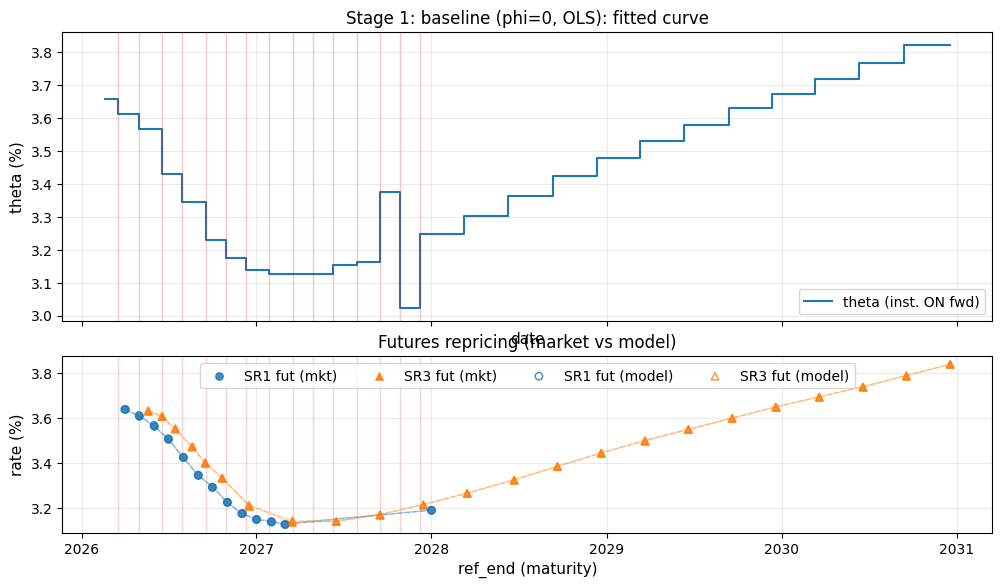
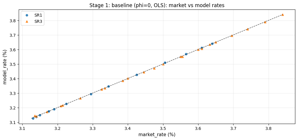
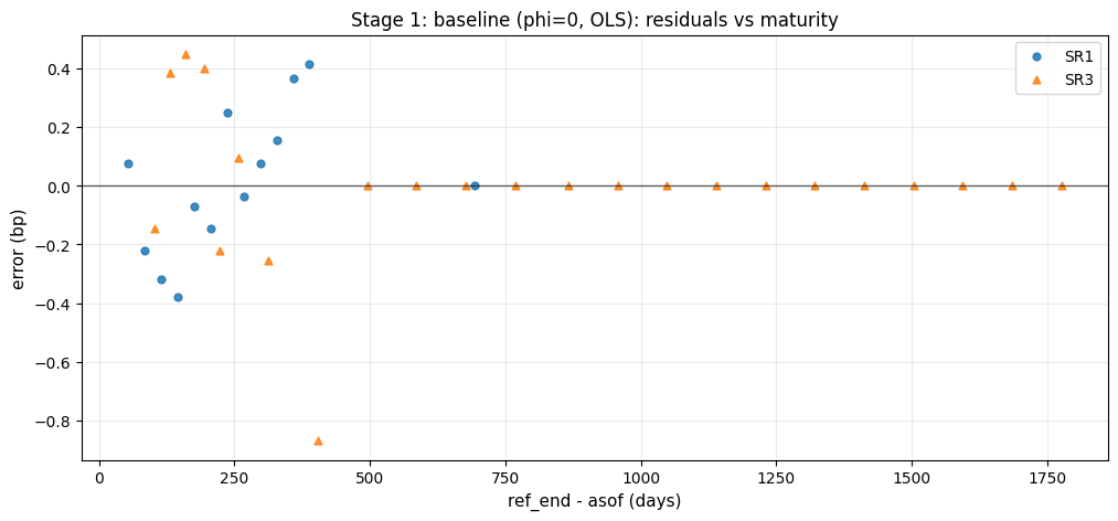
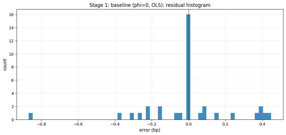
- Starting point (no previous stage): OLS, uniform weights, φ=0 (no smoothing), no realized fixings, simple knot grid.
Math (this stage)
\[\theta^{(1)}=\arg\min_\theta \sum_i \varepsilon_i(\theta)^2\]
This stage establishes a minimal, fully data-driven curve under SR1/SR3 pricing conventions. It is intentionally flexible, which makes it a good baseline but also a useful reference for identifying where later constraints (turn knots, smoothing, weighting, robust loss) materially change the fitted shape.
Residual diagnostics (Stage 1)
Interactive curve over time
What changed vs previous stage
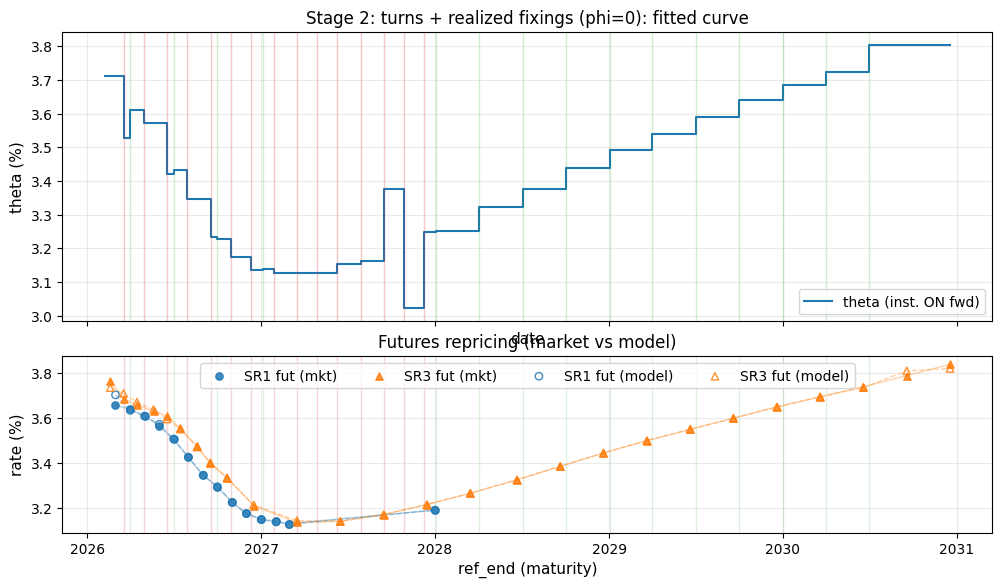
- Add quarter/year-end “turn” knots.
- Include realized SOFR fixings for in-progress contracts.
- Keep OLS, uniform weights, φ=0.
Key change (realized fixings)
\[r_{i,j}(\theta)= r^{fix}_{i,j}\ \text{if date} \le \text{last fixing date},\ \text{else}\ \theta_{k(i,j)}\]
This stage improves short-dated realism: once a contract has partially accrued, the realized portion should not be “re-fit” by the forward curve. Adding turn knots also gives the curve explicit degrees of freedom where the market often prices discontinuities (quarter-ends / year-ends).

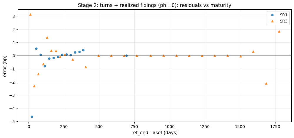
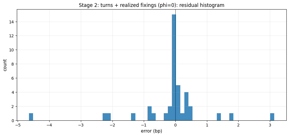
Residual diagnostics (Stage 2)
Interactive curve over time
What changed vs previous stage
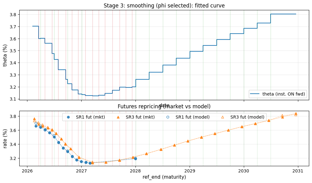
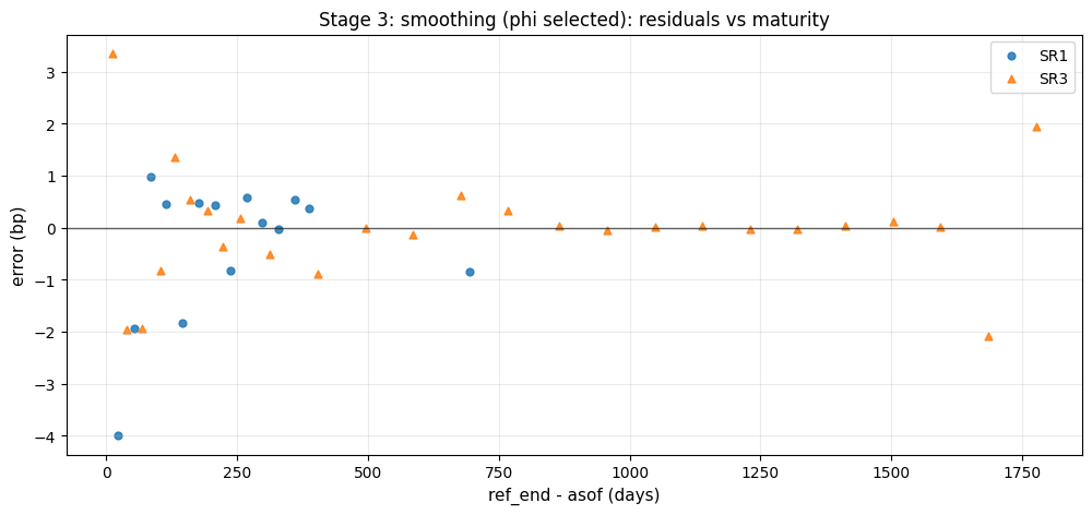
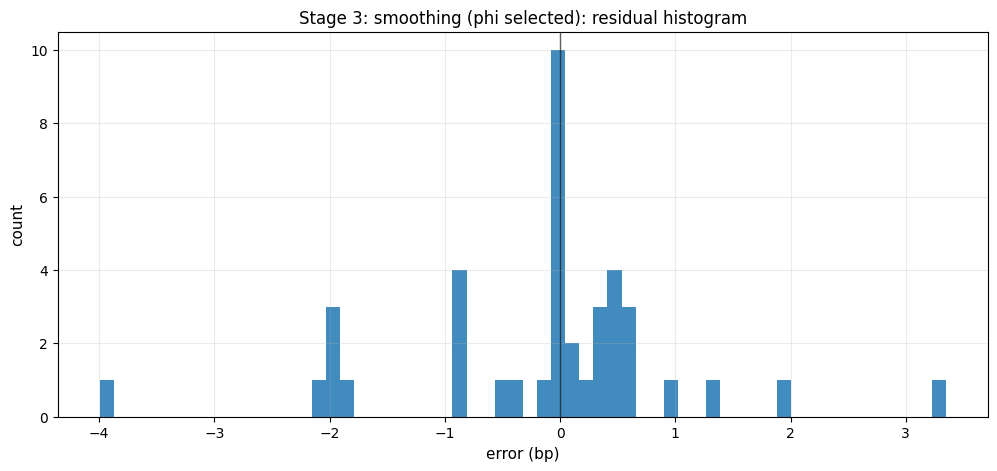
- Keep Stage 2 grid, add butterfly smoothness penalty.
- Choose φ via a scan.
Math (this stage)
\[\theta^{(3)}=\arg\min_\theta \left[\sum_i w_i^{eff}\varepsilon_i(\theta)^2 + \phi\sum_k b_k(\theta)^2\right]\]
\[b_k(\theta) = 100\,(2\theta_k - \theta_{k-1} - \theta_{k+1})\quad (\text{bp})\]
The smoothness term trades off local curve “wiggles” against repricing error. We choose φ via a simple scan (reported in the stage tables above): as φ rises, RMSE typically degrades slowly at first while roughness drops materially; beyond a point, φ over-smooths and fit quality deteriorates.
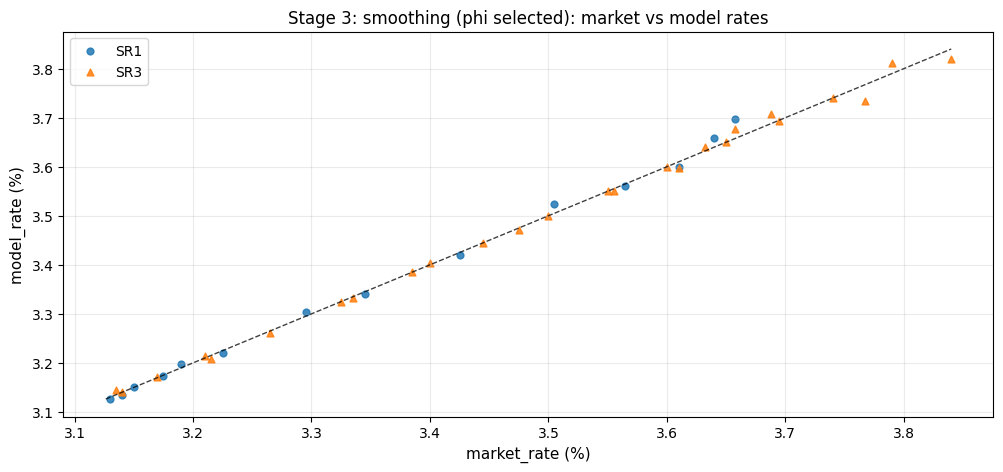
Residual diagnostics (Stage 3)
Interactive curve over time
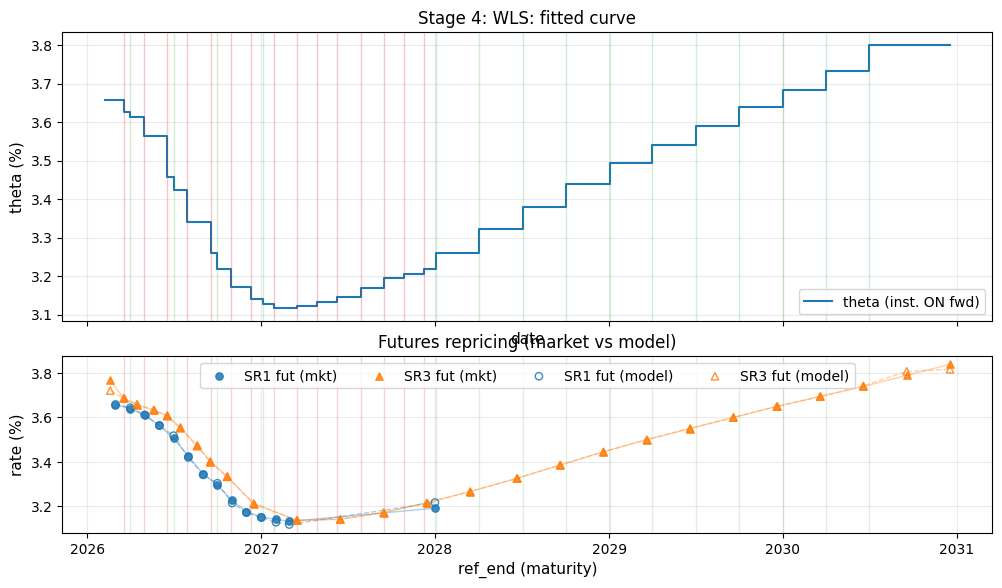
What changed vs previous stage
- Keep Stage 3, add liquidity weights (default
vol_x_oi).
Example weighting
\[\text{raw}_i = \sqrt{\text{volume}_i \cdot \text{open\_interest}_i}\]
\[w_i=\text{clip}\left(\frac{\text{raw}_i}{\text{median}(\text{raw}_j\ \text{within same root})},\ w_{min},\ w_{max}\right)\]
This stage reduces the influence of thin or noisy instruments: the curve prioritizes fitting liquid contracts and allows less-liquid points to deviate when they conflict with the broader surface. It’s a practical step toward stability when using the curve downstream (risk, carry/roll, relative value).
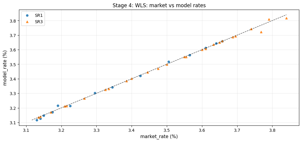
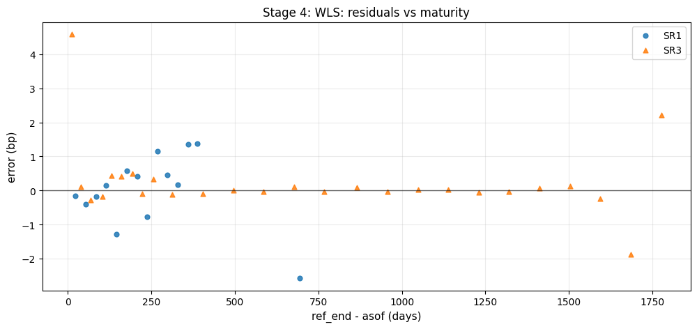
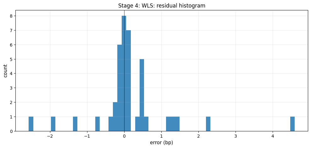
Residual diagnostics (Stage 4)
Interactive curve over time
What changed vs previous stage
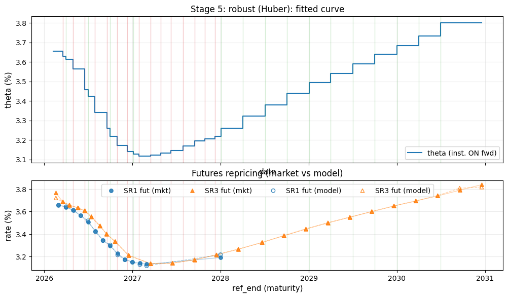
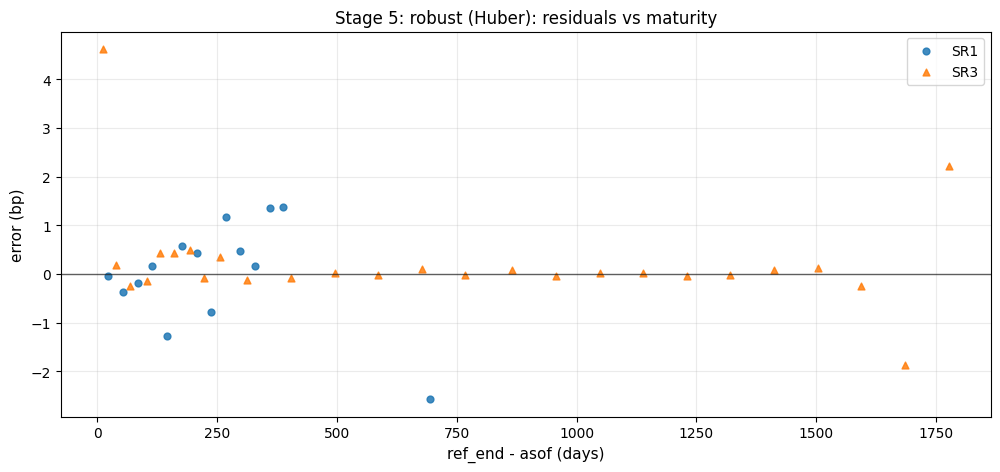
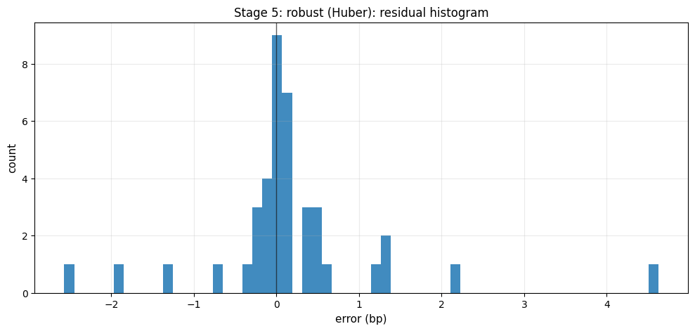
- Keep Stage 4, switch to Huber robust loss.
Define stacked residual vector
\[r(\theta) = \left[\sqrt{w_i^{eff}}\varepsilon_i(\theta)\right]_i \ \oplus\ \left[\sqrt{\phi}\,b_k(\theta)\right]_k\]
Optimize
\[\theta^{(5)} = \arg\min_\theta \sum_j \rho\left(\frac{r_j(\theta)}{s}\right)\]
Huber
\[\rho(u)=0.5u^2\ \text{if }|u|\le 1,\quad =|u|-0.5\ \text{if }|u|>1\]
This final stage keeps the same modeling structure but reduces sensitivity to outliers and occasional “bad” settlements. In practice, the curve tends to become more stable day-to-day, with outliers absorbed by the robust loss rather than by localized kinks in θ.
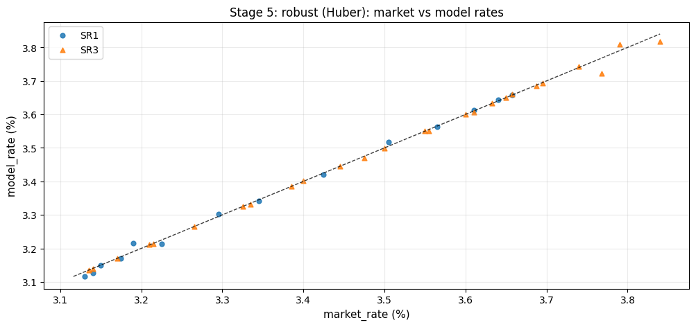
Residual diagnostics (Stage 5)
Interactive curve over time
Limitations and extensions
- Instrument set: SR1/SR3 futures cover only up to listed maturities; extrapolation beyond the last contract is not directly identified without additional instruments or priors.
- Day-count / calendar details: the fit depends on precise cash-business-day anchoring and holiday conventions; calendar mismatches show up first in short-dated contracts.
- Regularization choice: a step function plus second-difference smoothing is simple and robust, but other parameterizations (splines, monotone constraints, or stochastic-process priors) may be preferable for certain downstream uses.
- Uncertainty: the report focuses on a point estimate. Extensions could include bootstrapped/parametric uncertainty bands, stress scenarios, or diagnostics by contract bucket.