Fixed income relative value mean reversion

PCA-neutral Treasury butterfly backtest and PC3 mean reversion diagnostics.

Notebook: rv_project.ipynb

About the project

I’ve recently read a couple of interesting posts about fixed income RV on X. So interesting, that I’ve decided to take a shot at some fixed income RV modelling. This is my first project in this field, so obviously it might lack some desk-specific techniques that one would learn on the job. Practice is the best teacher, and since I’m not working on the RV desk this is my practice :)

Executive summary

This project builds a US Treasury curve relative value backtest that isolates curve shape risk by neutralizing the first two PCA factors on the traded legs and trading deviations in a PC3 normalized residual.

1. Universe and trade object: fit PCA on an eight tenor Treasury curve, then trade a three leg butterfly, default 2 year, 5 year, 10 year.
2. Signal: compute the hedged residual return from daily PCA neutral weights, cumulate it into a cumulative residual series, standardize it with a rolling z-score, enter whenever | z | >= 2
3. Headline full sample results: expanding net Sharpe is -0.115108 with annualized return -0.2252 percent, annualized volatility 1.9560 percent, max drawdown -17.3012 percent, and average turnover 0.0630. Rolling net Sharpe is -0.116290 with annualized return -0.2464 percent, annualized volatility 2.1190 percent, max drawdown -21.2617 percent, and average turnover 0.0732.
4. Key takeaway: Trading mean reversion in PC3 in a simple way like this does bring in positive returns, and while the strategy performed OK at the beginning, it underperforms post 2000. Also, since PC3 accounts for relatively little variance, the annualized vol of this strategy is very low – trading similar strategy should probably be done using leverage.
5. Implementation note: PnL is a duration scaled yield change proxy and ignores carry, rolldown, convexity, financing, and execution. Section 12 outlines a mapping to futures or swaps plus a more realistic cost and carry model.

1. High level hypothesis and factor model

Daily movements of the Treasury yield curve are well described by a small number of systematic factors. By constructing a portfolio that is neutral to the dominant components (level and slope), the remaining exposure isolates higher order curve dynamics that are often less persistent than level moves, which motivates a mean reversion style signal.

The strategy focuses on the third principal component because the variance explained by successive curve factors decays rapidly. The first component typically captures the bulk of variance and often corresponds to parallel level shifts. The second typically captures a smaller but still dominant share and often corresponds to slope changes. By the time we reach the third component, the explained variance is materially lower and the factor is no longer a primary driver of directional rate risk.

I formalize that intuition with a factor model on tenor returns. Let \(N\) be the number of tenors in the chosen curve universe, and let \(r_{t} \in \mathbb{R}^N\) be the duration scaled yield change return proxy vector at date \(t\). A generic factor model is

\[ r_{t} = B_{t} f_{t} + \varepsilon_{t} \]

where \(B_{t} \in \mathbb{R}^{N \text{ x } K}\) is a loading matrix, \(f_{t} \in \mathbb{R}^K\) is a factor return vector, and \(\varepsilon_{t}\) is the residual. In this project, \(B_{t}\) is estimated by PCA in a walk forward way, with \(K = 3\).

The trading object is a portfolio weight vector \(w_{t} \in \mathbb{R}^N\) such that the portfolio return

\[ r_{t}^{\mathrm{res}} = w_{t}^\top r_{t} \]

is neutral to the dominant factors. In implementation, \(w_t\) is sparse: only three butterfly legs are nonzero and the other tenor weights are exactly zero. This is because if we treat factors past PC1-PC3 as residual, we can achieve our desired exposure to PC1-PC3 using only three instruments.

2. Data Audit

I began by loading the wide macro dataset panel stored at:

data/combined/all_datasets_wide.parquet

The initial goal was not examine the data and see what it can support without calendar artifacts, hidden interpolation, or silent missingness.

I ran three checks that determined the rest of the project:

1. Column inventory and grouping to verify what series exist and how they cluster
2. Era coverage tables to find stable windows where a complete curve is available
3. Frequency diagnostics to identify series that are not daily and should not be mixed into a daily backtest without care

Table 1: Data audit column inventory and group summary

column_name	group	dtype	start_date	end_date	obs_count	missing_percent
DGS1	fred_dgs	float64	1962-01-02	2026-01-15	15994	4.279131
DGS10	fred_dgs	float64	1962-01-02	2026-01-15	15994	4.279131
DGS20	fred_dgs	float64	1962-01-02	2026-01-15	14305	14.387456
DGS3	fred_dgs	float64	1962-01-02	2026-01-15	15994	4.279131
DGS5	fred_dgs	float64	1962-01-02	2026-01-15	15994	4.279131
DGS7	fred_dgs	float64	1969-07-01	2026-01-15	14124	15.470704
DGS2	fred_dgs	float64	1976-06-01	2026-01-15	12402	25.776528
DGS30	fred_dgs	float64	1977-02-15	2026-01-15	12224	26.841822
DGS3MO	fred_dgs	float64	1981-09-01	2026-01-15	11092	33.616614
DGS6MO	fred_dgs	float64	1981-09-01	2026-01-15	11092	33.616614
DGS1MO	fred_dgs	float64	2001-07-31	2026-01-15	6116	63.396972
eurofx	macro	float64	1999-01-04	2026-01-09	6776	59.447005
fed_assets	macro	float64	2002-12-18	2026-01-14	1205	92.788318
tga	macro	float64	2002-12-18	2026-01-14	1205	92.788318
rrp	macro	float64	2003-02-07	2026-01-16	3161	81.082052
10_yr	treasury_par_curve	float64	1990-01-02	2026-01-16	9016	46.041056
1_yr	treasury_par_curve	float64	1990-01-02	2026-01-16	9016	46.041056
2_yr	treasury_par_curve	float64	1990-01-02	2026-01-16	9016	46.041056
30_yr	treasury_par_curve	float64	1990-01-02	2026-01-16	8022	51.989946
3_mo	treasury_par_curve	float64	1990-01-02	2026-01-16	9013	46.059010
3_yr	treasury_par_curve	float64	1990-01-02	2026-01-16	9016	46.041056
5_yr	treasury_par_curve	float64	1990-01-02	2026-01-16	9016	46.041056
6_mo	treasury_par_curve	float64	1990-01-02	2026-01-16	9016	46.041056
7_yr	treasury_par_curve	float64	1990-01-02	2026-01-16	9016	46.041056
20_yr	treasury_par_curve	float64	1993-10-01	2026-01-16	8077	51.660782
1_mo	treasury_par_curve	float64	2001-07-31	2026-01-16	6117	63.390987
2_mo	treasury_par_curve	float64	2018-10-16	2026-01-16	1812	89.155545
4_mo	treasury_par_curve	float64	2022-10-19	2026-01-16	810	95.152313
15_month	treasury_par_curve	float64	2025-02-18	2026-01-16	229	98.629481

Table 2: Availability snapshot by era for key groups

era	group	days_in_index	any_non_null_days	any_non_null_pct
pre_2008	treasury_par_curve	4695	4503	0.959105
post_2008	treasury_par_curve	3131	3002	0.958799
post_2020	treasury_par_curve	1578	1511	0.957541
pre_2008	fred_dgs	4695	4503	0.959105
post_2008	fred_dgs	3131	3002	0.958799
post_2020	fred_dgs	1578	1510	0.956907
pre_2008	macro	4695	2268	0.483067
post_2008	macro	3131	3020	0.964548
post_2020	macro	1578	1520	0.963245

Decision
The audit made it clear that a curve strategy needs its own clean, canonical curve panel. Without that, PCA and any walk forward estimation would be unstable for reasons unrelated to markets.

3. Canonical curve panel

I focused on Treasury par yield curve data stored at:

data/single_assets/treasury_par_yield_curve.parquet

The raw curve is not guaranteed to be on a perfectly regular calendar, and some tenors have structural gaps. If I fit PCA on a panel that fabricates missing observation dates, I will end up modeling missingness mechanics rather than curve dynamics.

So I built a canonical curve panel with explicit rules:

1. Standardize column names to a consistent tenor schema such as 3_mo, 2_yr, 10_yr
2. Select a candidate tenor set and verify it exists in the raw dataset
3. Create a canonical trading calendar from observed curve dates and reindex the curve to it
4. Save the canonical panel plus an audit manifest for reproducibility
5. Produce diagnostics that summarize missingness on the observed trading calendar

Key output artifacts:

1. data/derived/curve_treasury_par_canonical.parquet
2. data/derived/curve_treasury_par_canonical_manifest.parquet
3. data/derived/curve_missingness_summary.parquet
4. data/derived/curve_missing_streaks_long_end.parquet
5. data/derived/curve_universe_feasibility.parquet
6. data/derived/curve_universe_recommendation.parquet

3.1 PCA structure diagnostics on yield changes

To document the factor structure of the canonical curve through time, I run PCA on daily yield changes in basis points for the main eight tenor universe. I report rolling explained variance ratios and loading shapes at several snapshot dates.

Key output artifacts:

1. outputs/section_03/pca_evr_rolling_5y.csv
2. outputs/section_03/pca_evr_rolling_5y.png
3. outputs/section_03/pca_snapshots_explained_variance.csv
4. outputs/section_03/pca_snapshots_loadings.csv
5. outputs/section_03/pca_loadings_snapshots.png

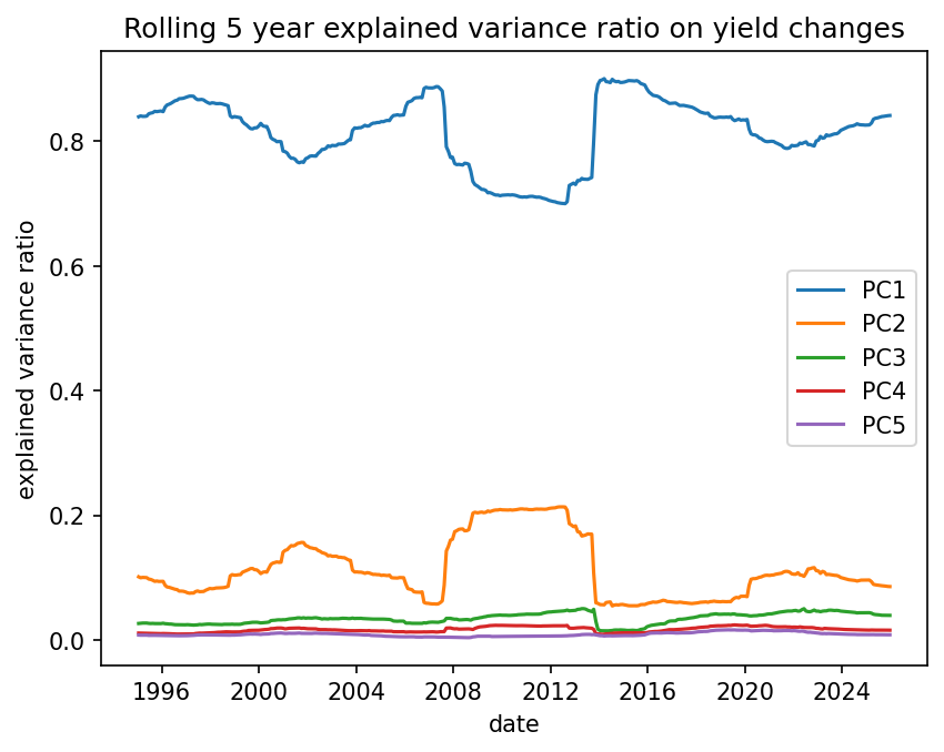
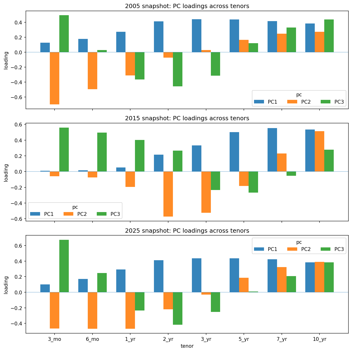
Table 3: Universe feasibility table using overlap dates

universe	n_cols	first_date_all_non_null	last_date_all_non_null	n_days_all_non_null	share_of_overlap_days	missing_pct_on_overlap
U_core_8	8	1990-01-02	2026-01-16	9013	0.999556	0.015249
U_core_9	9	1990-01-02	2026-01-16	8019	0.889320	1.239634
U_core_10	10	1993-10-01	2026-01-16	7080	0.785184	2.158146
U_short_end	5	2001-07-31	2026-01-16	6114	0.678053	6.447821

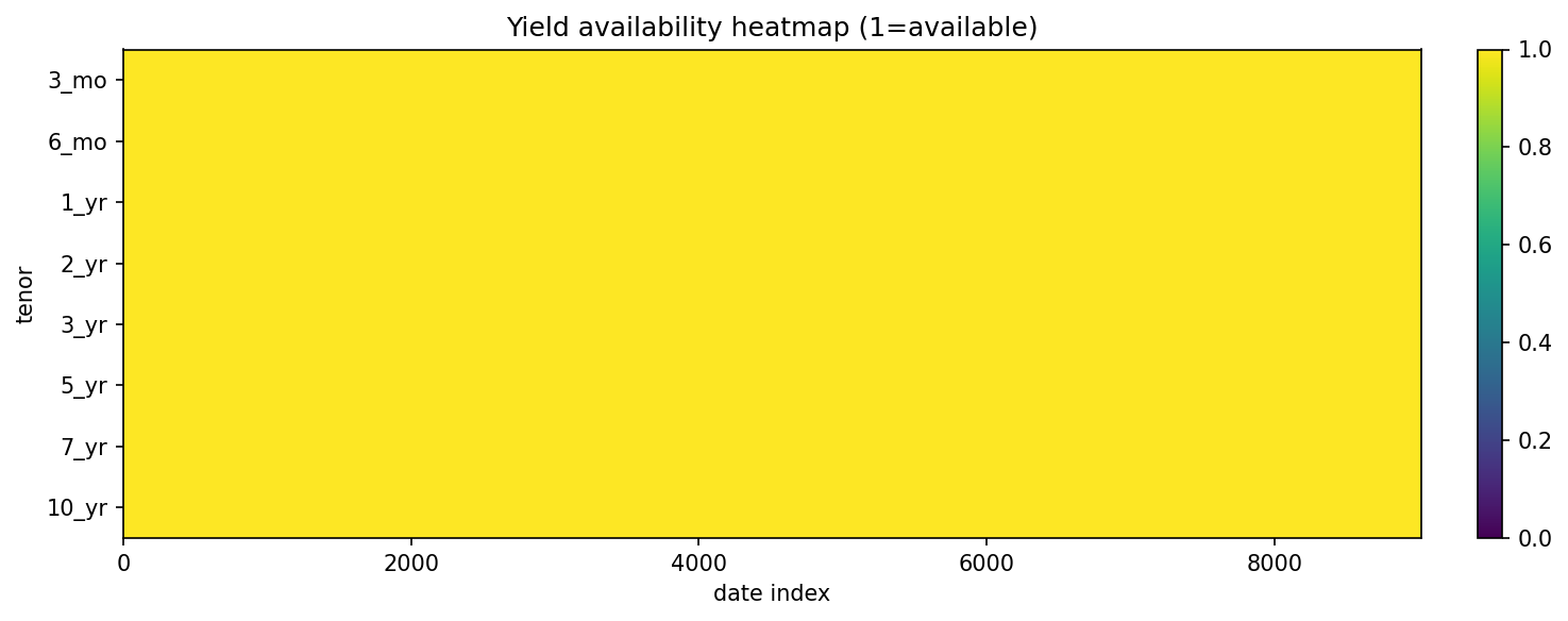
What I learned and how it changed the plan: the long end is the limiting factor. Because a relative value strategy needs a stable trading calendar, I chose a core universe that remains continuously available.

Decision
Universe name: U_core_8
Tenors: 3_mo, 6_mo, 1_yr, 2_yr, 3_yr, 5_yr, 7_yr, 10_yr

This avoids backtests that implicitly condition on data availability, which can create bias.

4. Backtest specification

Once the universe was fixed, I wrote down a backtest specification that every downstream step must respect. The purpose is to make the research easy to audit and hard to accidentally contaminate with look ahead.

The specification has three parts:

1. The trading calendar
2. The PnL proxy conventions
3. The timing conventions for estimation and trading

4.1 Trading calendar via overlap dates

The canonical panel is derived from the raw curve, but their calendars can differ. To avoid silent misalignment, I define the trading calendar as the intersection of raw curve dates and canonical curve dates, then restrict to the window where all chosen tenors are non null.

Table 4: Sample window summary for overlap and all non null dates

field	value
universe_name	U_core_8
tenors	3_mo, 6_mo, 1_yr, 2_yr, 3_yr, 5_yr, 7_yr, 10_yr
overlap_start_date	1990-01-02
overlap_end_date	2026-01-16
n_overlap_dates	9017
sample_start_all_non_null	1990-01-02
sample_end_all_non_null	2026-01-16
n_days_all_non_null	9013

4.2 Duration scaled yield change return proxy from yield changes

The strategy works on a return proxy rather than on yield levels. Yields are stored in percent. For tenor \(i\), define the daily yield change in percent points:

\[ d y_{t,i} = y_{t,i} - y_{t-1,i}. \]

Convert yield changes to decimal units:

\[ d y_{t,i}^{\text{dec}} = \frac{d y_{t,i}}{100}. \]

Yield changes are then mapped into a duration scaled yield change return proxy using approximate modified durations computed from the observed yields under the par bond assumptions in the notebook. The duration applied to the date \(t\) return proxy is lagged by one observation, so \(D_{t-1,i}\) is applied to \(d y_{t,i}^{\text{dec}}\). For tenor (i), the proxy return is defined as

\[ r_{t,i} = - D_{t-1,i} \, d y_{t,i}^{\text{dec}}. \]

Here \(D_{t-1,i}\) denotes the modified duration proxy in years. The output \(r_{t,i}\) is dimensionless and should be read as a first order price return proxy from yield changes, not as a dollar DV01 and not as a tradeable instrument PnL. In practice, actual dollar DV01 depends on coupon, yield level, convexity, instrument choice, and position sizing. But since this is the data we have, we’ll roll with it.

Unit check with a concrete example: if \(D_{t-1,i} = 5\) years and the yield rises by 1 bp, then \(d y_{t,i}^{\text{dec}} = 0.0001\) and \(r_{t,i} \simeq -5 \cdot 0.0001 = -0.0005\), which is about -5 bp in price return terms.

Table 5: Approximate modified duration summary used for duration scaling (median across the sample)

tenor	maturity_years	duration_years	duration_mean	duration_p05	duration_p95
3_mo	0.25	0.243404	0.243326	0.235938	0.249925
6_mo	0.50	0.485437	0.486113	0.470633	0.499700
1_yr	1.00	0.969838	0.971307	0.940734	0.998901
2_yr	2.00	1.919327	1.922656	1.839596	1.994014
3_yr	3.00	2.822107	2.831280	2.659034	2.981190
5_yr	5.00	4.524370	4.529618	4.102283	4.896069
7_yr	7.00	6.070200	6.067327	5.330713	6.702224
10_yr	10.00	8.109048	8.127441	6.852685	9.225822

4.3 Timing conventions to avoid look ahead

I enforce a strict rule: signals and weights used at date \(t\) are computed using information available through \(t-1\), while PCA refits use data through \(t\) at end-of-day \(t\).

Operationally:

1. PCA loadings, means, and hedge weights are forward-filled to the daily trading calendar and shifted by one observation, so the trade date uses the most recent refit date \(\le t-1\)
2. Z-score statistics use trailing windows computed at the close, so \(z_t\) is based on data through \(t\)
3. The state machine uses the prior day z-score (\(z_{t-1}\)) to decide entry and exit, so trade decisions use information through the prior close

Key output artifact: data/derived/backtest_spec.json

5. Walk forward PCA and portfolio

With a clean panel and timing rules fixed, I moved to modeling. The objective is to construct a residual portfolio that is neutral to PCs 1 and 2.

5.1 PCA on centered return panels

Let \(R \in \mathbb{R}^{T \text{ x } N}\) be the return matrix over a single PCA fit window of length \(T\), where each row is \(r_{t}^\top\) for \(t\) in that fit window. I center the columns using the mean computed only within this fit window:

\[ R_{c} = R - \mathbf{1}\mu^\top \quad \mu = \frac{1}{T}\sum_{t=1}^T r_{t} \]

Note: \(\mu\) is the fit window mean. It is recomputed at each refit using only the \(T\) observations in the current window (the dependence of \(\mu\) on the window is suppressed in the notation). It is not a full sample mean.

I then compute an SVD:

\[ R_{c} = U \Sigma V^\top \]

The first \(K\) right singular vectors give the PCA loading vectors. For \(K=3\), define

\[ B = \begin{bmatrix} v_{1} & v_{2} & v_{3} \end{bmatrix} \in \mathbb{R}^{N \text{ x } 3} \]

where \(v_k\) is the \(k\) th loading vector over the fit window. The corresponding factor returns are

\[ f_{t} = B^\top (r_{t} - \mu) \]

5.2 Walk forward refit schedule

Curve regimes change. So I estimate PCA in a walk forward way. I implement two modes:

1. Expanding window: the fit sample grows over time
2. Rolling window: the fit sample has a fixed length

Refits occur every 21 observations on the curve trading calendar. The default rolling window length is 756 observations.

Table 6: PCA refit schedule for expanding and rolling modes

Expanding schedule preview

refit_date	mode	window_start_date	window_end_date	n_obs_in_window	refit_step_obs
1991-01-04	expanding	1990-01-03	1991-01-04	252	<NA>
1991-02-05	expanding	1990-01-03	1991-02-05	273	21
1991-03-07	expanding	1990-01-03	1991-03-07	294	21
1991-04-08	expanding	1990-01-03	1991-04-08	315	21
1991-05-07	expanding	1990-01-03	1991-05-07	336	21
…	…	…	…	…	…
2025-09-10	expanding	1990-01-03	2025-09-10	8925	21
2025-10-09	expanding	1990-01-03	2025-10-09	8946	21
2025-11-10	expanding	1990-01-03	2025-11-10	8967	21
2025-12-11	expanding	1990-01-03	2025-12-11	8988	21
2026-01-13	expanding	1990-01-03	2026-01-13	9009	21

Rolling schedule preview

refit_date	mode	window_start_date	window_end_date	n_obs_in_window	refit_step_obs
1993-01-11	rolling	1990-01-03	1993-01-11	756	<NA>
1993-02-10	rolling	1990-02-02	1993-02-10	756	21
1993-03-12	rolling	1990-03-06	1993-03-12	756	21
1993-04-13	rolling	1990-04-04	1993-04-13	756	21
1993-05-12	rolling	1990-05-04	1993-05-12	756	21
…	…	…	…	…	…
2025-09-10	rolling	2022-08-31	2025-09-10	756	21
2025-10-09	rolling	2022-09-30	2025-10-09	756	21
2025-11-10	rolling	2022-11-01	2025-11-10	756	21
2025-12-11	rolling	2022-12-02	2025-12-11	756	21
2026-01-13	rolling	2023-01-04	2026-01-13	756	21

5.3 Loading stability diagnostics

PCA loadings can flip sign without changing the underlying subspace. Between refits, I align signs and track similarity diagnostics so that the hedge portfolio does not churn purely from sign ambiguity.

A simple similarity score between two loadings \(v\) and \(\tilde v\) is the absolute cosine similarity:

\[ \mathrm{sim}(v,\tilde v) = \left|\frac{v^\top \tilde v}{\lVert v \rVert \lVert \tilde v \rVert}\right| \]

This is part of an internal diagnostic table persisted during the run.

Table 7: PCA stability diagnostics

Preview rows

refit_date	sim1	sim2	sim3	gap12	gap23	perm_used	flip_pc1	flip_pc2	flip_pc3	freeze_event
1991-01-04	NaN	NaN	NaN	0.948420	0.013775	0-1-2	False	False	False	False
1991-02-05	0.999976	0.998323	0.998851	0.943845	0.016010	0-1-2	True	True	True	False
1991-03-07	0.999999	0.999493	0.999143	0.940057	0.017306	0-1-2	True	True	True	False
1991-04-08	0.999995	0.999980	0.999985	0.939805	0.017607	0-1-2	True	True	True	False
1991-05-07	0.999998	0.999903	0.999463	0.939546	0.017350	0-1-2	True	True	True	False
1991-06-06	0.999998	0.999947	0.999543	0.937401	0.017965	0-1-2	True	True	True	False
1991-07-08	0.999996	0.999915	0.999470	0.936457	0.017975	0-1-2	True	True	True	False
1991-08-06	0.999994	0.999964	0.999303	0.936635	0.017672	0-1-2	True	True	True	False
1991-09-05	0.999993	0.999935	0.999515	0.934205	0.018890	0-1-2	True	True	True	False
1991-10-04	0.999999	0.999992	0.999932	0.933744	0.018728	0-1-2	True	True	True	False
1991-11-05	0.999998	0.999970	0.999217	0.934197	0.018373	0-1-2	True	True	True	False
1991-12-06	0.999997	0.999971	0.999994	0.931956	0.019240	0-1-2	True	True	True	False

Summary

refits	sim3_p05	sim3_min	freeze_events
418	0.99984	0.998819	0

5.4 Solving hedge weights by enforcing factor neutrality constraints

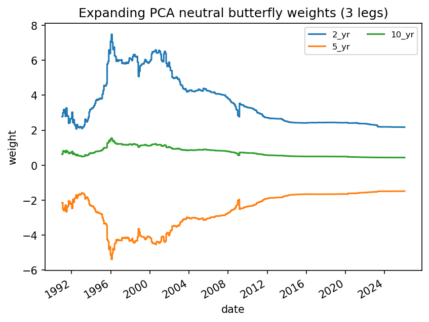
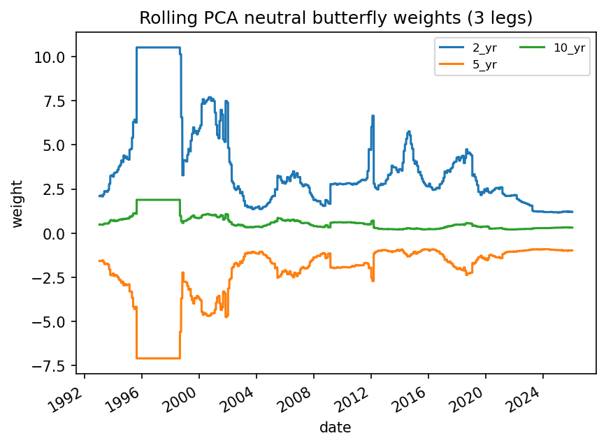
This project keeps the PCA fit on the full 8 tenor curve, but it trades a three leg butterfly to reduce rebalancing. The butterfly legs are configured as ["2_yr","5_yr","10_yr"] by default.

At each refit date \(\tau\), I compute PCA loadings on the full return panel, producing \(L_{k}(\tau) \in \mathbb{R}^{N}\) for \(k \in \{1,2,3\}\). Instead of trading weights across all \(N\) tenors, I restrict the trade to three tenors \(i_1,i_2,i_3\) and solve only for a 3 vector \(w_{\mathrm{leg}}(\tau) \in \mathbb{R}^{3}\).

Define the leg restricted loading matrix

\[ A_{\mathrm{leg}}(\tau)= \begin{bmatrix} L_{1}(\tau)_{i_1} & L_{1}(\tau)_{i_2} & L_{1}(\tau)_{i_3} \\ L_{2}(\tau)_{i_1} & L_{2}(\tau)_{i_2} & L_{2}(\tau)_{i_3} \\ L_{3}(\tau)_{i_1} & L_{3}(\tau)_{i_2} & L_{3}(\tau)_{i_3} \end{bmatrix} \in \mathbb{R}^{3 \text{ x } 3}. \]

I then solve the PCA neutral butterfly constraints on those three legs:

\[ A_{\mathrm{leg}}(\tau)\, w_{\mathrm{leg}}(\tau) = \begin{bmatrix} 0 \\ 0 \\ 1 \end{bmatrix}. \]

This enforces PC1 and PC2 neutrality on the traded legs, while normalizing the butterfly to have unit exposure to PC3 on the refit date. I embed these three weights into a full \(w(\tau) \in \mathbb{R}^N\) by setting all non leg tenors to zero, so downstream residual construction continues to work on the full tenor list without special casing.

Implementation guardrail: the leg restricted system can become ill conditioned or produce extreme leverage. If \(\kappa\!\left(A_{\mathrm{leg}}(\tau)\right)\) exceeds butterfly_max_cond (default 200), or if the leg weights breach butterfly_max_l1 or butterfly_max_abs, the code keeps the previous refit weights and records a freeze event rather than applying an unstable solve.

5.5 Daily weights with one observation shift

Weights are solved on refit dates, then forward filled across trade dates and shifted by 1 observation to enforce causality:

\[ w_{t} = w\!\left(\tau(t-1)\right) \]

where \(\tau(t-1)\) is the most recent refit date at or before \(t-1\).

Key output artifacts include:

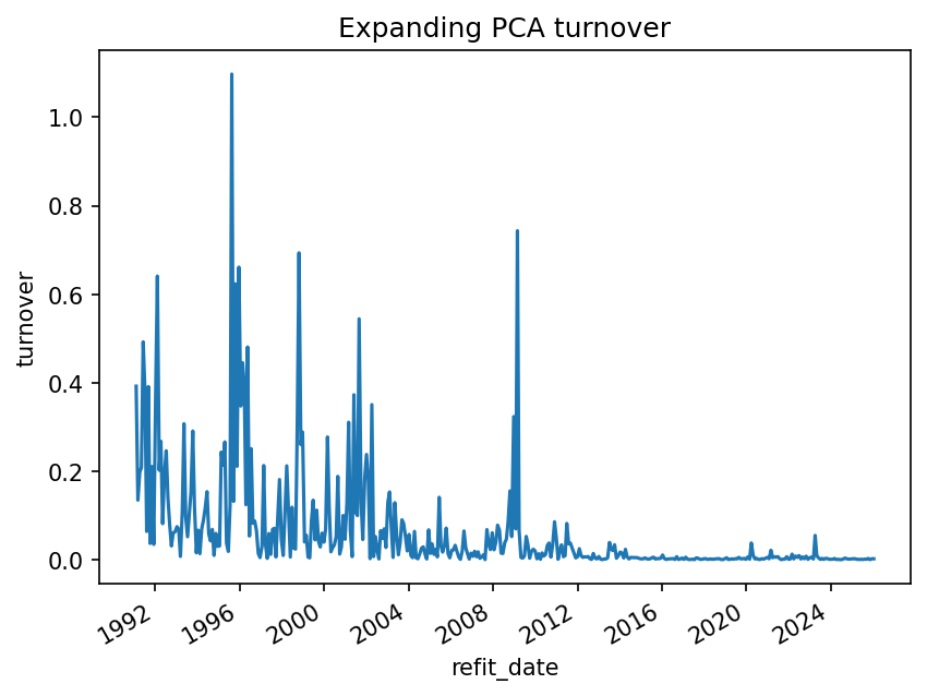
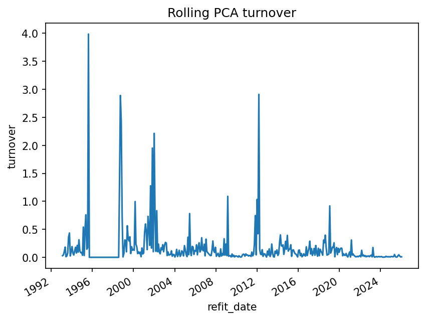
1. data/derived/pca_weights_refit_expanding.parquet
2. data/derived/pca_turnover_expanding.parquet
3. data/derived/pca_weights_daily_expanding.parquet
4. data/derived/pca_loadings_daily_expanding.parquet
5. data/derived/pca_weights_refit_rolling.parquet
6. data/derived/pca_turnover_rolling.parquet
7. data/derived/pca_weights_daily_rolling.parquet
8. data/derived/pca_loadings_daily_rolling.parquet

The daily weights table contains all 8 tenor columns for alignment and auditability, but only the butterfly legs are nonzero. This makes the trade object explicit and keeps turnover localized to three instruments instead of spreading small changes across the entire curve panel.

6. Residual and standardized signal

Once daily hedge weights exist, the strategy becomes a signal processing pipeline.

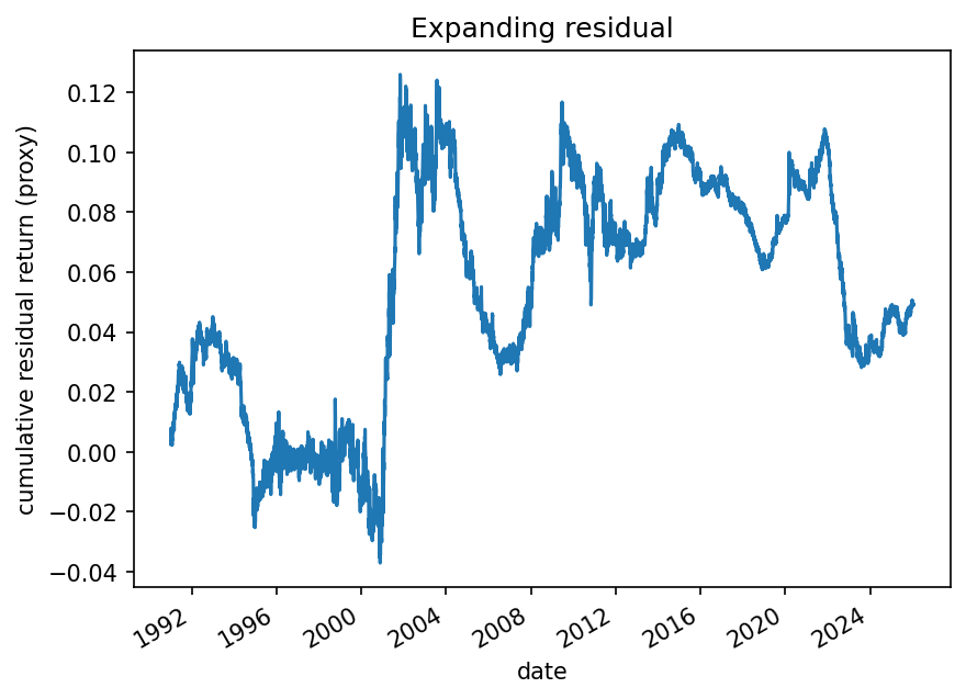
6.1 Residual return and cumulative residual

Define the residual portfolio return as the hedged return:

\[ r_{t}^{\mathrm{res}} = w_{t}^\top r_{t} \]

I convert this into a cumulative residual series by cumulation:

\[ s_{t} = \sum_{u \le t} r_{u}^{\mathrm{res}} \]

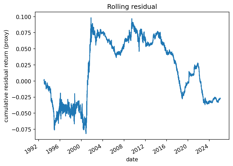
This is the object I standardize into a z score. This cumulative residual is a constructed state variable for standardization and is not an instrument price level. The cumulation is deliberate: in many relative value contexts, deviations are more stable to model in levels than in raw returns.

Key output artifacts:

1. data/derived/residual_expanding.parquet
2. data/derived/residual_rolling.parquet

6.2 Z score with trailing window statistics

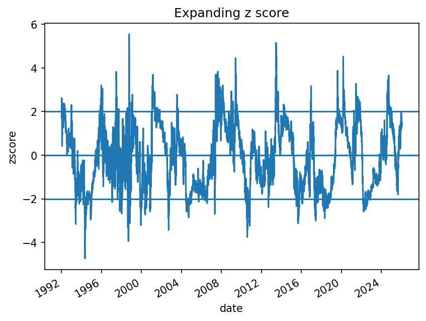
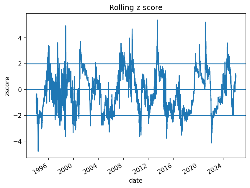
Let \(W\) be the z score window length, default 252 observations. Define trailing statistics that use information up to \(t\):

\[ m_{t} = \frac{1}{W}\sum_{j=0}^{W-1} s_{t-j}, \quad \sigma_{t} = \sqrt{\frac{1}{W}\sum_{j=0}^{W-1}(s_{t-j} - m_{t})^2} \]

Then the z score at date \(t\) is

\[ z_{t} = \frac{s_{t} - m_{t}}{\sigma_{t}} \]

In the implementation, \(m_{t}\) and \(\sigma_{t}\) are computed as rolling statistics at each close, while the trading state machine uses \(z_{t-1}\) so decisions use information through the prior close.

Key output artifacts:

1. data/derived/zscore_expanding.parquet
2. data/derived/zscore_rolling.parquet

6.3 Raw signal flags

The raw directional signal is

\[ \mathrm{signal}_{t}^{\mathrm{raw}} = \begin{cases} +1, & z_{t} \le - 2, \\ -1, & z_{t} \ge 2, \\ 0, & \text{otherwise}. \end{cases} \]

Key output artifacts:

1. data/derived/signal_flags_expanding.parquet
2. data/derived/signal_flags_rolling.parquet

6.4 Mean reversion diagnostics

I run simple stationarity and half life diagnostics on the cumulative residual series to check whether mean reversion is statistically plausible in the full sample. These tests are descriptive only: they summarize persistence over the full sample and do not guarantee stability across regimes.

Key output artifacts:

1. outputs/section_06/mean_reversion_tests.csv

variant	sample_start	sample_end	n_obs	adf_stat	adf_p	kpss_stat	kpss_p	ar1_phi	half_life_days
expanding	1991-01-07 00:00:00	2026-01-16 00:00:00	8756	-1.95249	0.307783	6.072	0.01	0.998698	532.194
rolling	1993-01-12 00:00:00	2026-01-16 00:00:00	8252	-1.10086	0.714728	3.15582	0.01	0.999228	897.683

These full sample diagnostics are concerning for the core mean reversion premise. The ADF test fails to reject a unit root while KPSS rejects stationarity, and the AR(1) persistence estimates are extremely close to one, implying half life estimates on the order of years. Taken at face value, this suggests the cumulative two factor residual behaves more like a drifting process than a stationary spread, which makes fixed threshold mean reversion trading structurally fragile and likely regime dependent. I continue the analysis anyway for two reasons. First, these tests are descriptive full sample summaries and can hide time variation, structural breaks, and pockets of stronger mean reversion in specific regimes. Second, part of the project goal is to demonstrate an end to end research process that remains auditable even when the initial hypothesis weakens, including careful timing conventions, walk forward estimation, stability guardrails, and diagnostics that can falsify the thesis.

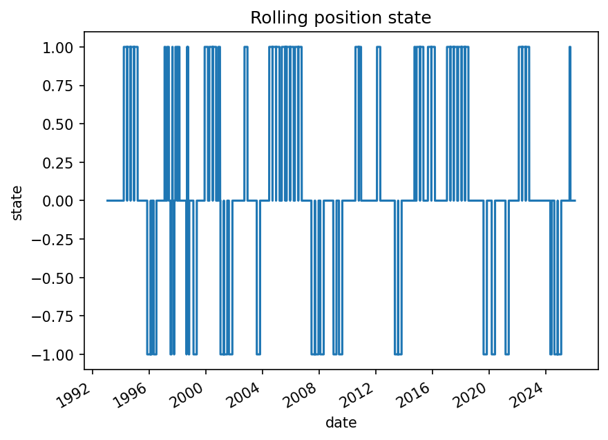
7. Trading logic

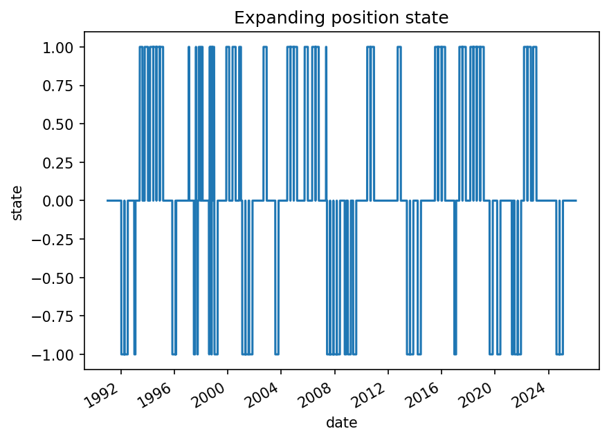
Let \(p_{t} \in { -1, 0, +1 }\) be the discrete position state at date \(t\). The trading logic uses the prior day z score, not the current day z score, to prevent same day look ahead.

Let \(z_{\mathrm{exit}} = 0.0\) and \(H_{\max} = 60\) observations by default.

Entry when flat:

\[ p_{t} = \begin{cases} +1, & p_{t-1}=0 \ \text{and}\ z_{t-1} \le -z_{\mathrm{entry}}, \\ -1, & p_{t-1}=0 \ \text{and}\ z_{t-1} \ge z_{\mathrm{entry}}, \\ 0, & p_{t-1}=0 \ \text{and otherwise}. \end{cases} \]

Exit when long:

\[ p_{t} = \begin{cases} 0, & p_{t-1}=+1 \ \text{and}\ (z_{t-1} \ge -z_{\mathrm{exit}} \ \text{or}\ h_{t-1} \ge H_{\max}), \\ +1, & p_{t-1}=+1 \ \text{and otherwise}. \end{cases} \]

Exit when short:

\[ p_{t} = \begin{cases} 0, & p_{t-1}=-1 \ \text{and}\ (z_{t-1} \le z_{\mathrm{exit}} \ \text{or}\ h_{t-1} \ge H_{\max}), \\ -1, & p_{t-1}=-1 \ \text{and otherwise}. \end{cases} \]

Here \(h_{t}\) is the holding day count tracked internally by the state machine, reset to zero when flat.

Note: trade_hit_rate is the fraction of profitable trades (trade-level), unlike hit_rate in the daily summary tables which is day-level and includes flat days as non-positive.

Table 8: Trade stats

variant	n_trades	trade_hit_rate	avg_hold_days	avg_abs_z_entry	p95_hold_days
expanding	72	0.486111	48.4306	2.27793	60
rolling	68	0.411765	48.4853	2.28344	60

8. Portfolio simulation, turnover, and costs

Once I have a discrete position state, I create a position vector over tenors:

\[ x_{t} = p_{t} \, w_{t}. \]

The gross daily PnL proxy is

\[ \mathrm{PnL}_{t}^{\mathrm{gross}} = x_{t}^\top r_{t}. \]

PnL at date \(t\) corresponds to yield changes from \(t-1\) to \(t\) because \(r_{t}\) is constructed from \(y_{t} - y_{t-1}\). A position chosen using the prior day signal is applied at date \(t\) and earns the date \(t\) return proxy.

Turnover is defined as

\[ \mathrm{TO}_{t} = \frac{1}{2}\lVert x_{t} - x_{t-1} \rVert_{1}. \]

Trading cost is linear in turnover:

\[ \mathrm{Cost}_{t} = c \, \mathrm{TO}_{t} \]

with default \(c = 10^{-4}\) (stored as parameter_defaults.cost_per_turnover in data/derived/backtest_spec.json). Net PnL is

\[ \mathrm{PnL}_{t}^{\mathrm{net}} = \mathrm{PnL}_{t}^{\mathrm{gross}} - \mathrm{Cost}_{t}. \]

Key output artifacts:

1. data/derived/bt_daily_expanding.parquet
2. data/derived/bt_trade_list_expanding.parquet
3. data/derived/bt_daily_rolling.parquet
4. data/derived/bt_trade_list_rolling.parquet

9. Performance and diagnostics

Once the backtest runs, the next question is whether the result is actually curve relative value or a disguised directional bet.

9.1 Equity curve and drawdown

I compute cumulative gross and net PnL proxy:

\[ \mathrm{Equity}_{t}^{\mathrm{net}} = \sum_{u \le t} \mathrm{PnL}_{u}^{\mathrm{net}} \]

Drawdown is computed from the running peak of that equity curve.

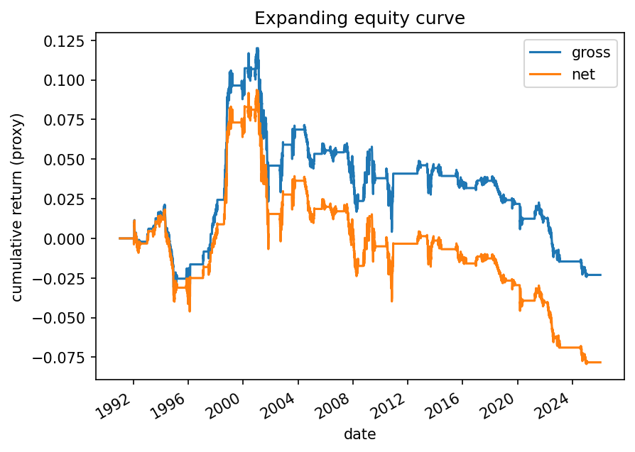
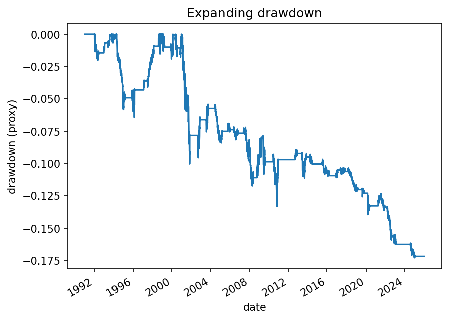
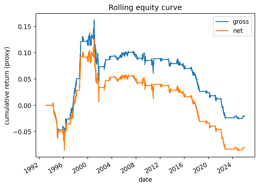
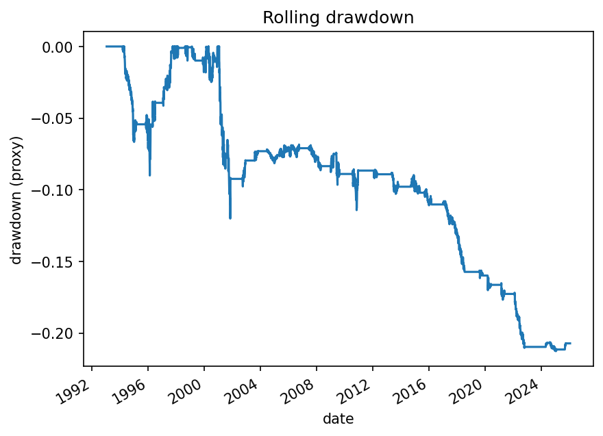
Table 9: Summary metrics

Interpretation note: hit_rate here is the daily fraction of positive PnL days (flat days count as non-positive).

variant	series	start	end	n_days	ann_ret	ann_vol	sharpe	hit_rate	max_drawdown	avg_turnover	var_95
expanding	gross	1991-01-07 00:00:00	2026-01-16 00:00:00	8756	-0.000664	0.019558	-0.033928	0.192325	-0.144349	0.063016	-0.001657
expanding	net	1991-01-07 00:00:00	2026-01-16 00:00:00	8756	-0.002252	0.01956	-0.115108	0.191754	-0.173012	0.063016	-0.001666
rolling	gross	1993-01-12 00:00:00	2026-01-16 00:00:00	8252	-0.000619	0.021194	-0.02919	0.19365	-0.188303	0.073233	-0.00162
rolling	net	1993-01-12 00:00:00	2026-01-16 00:00:00	8252	-0.002464	0.02119	-0.11629	0.192559	-0.212617	0.073233	-0.001629

Table 10: Drawdown episodes

The table below reports drawdown episodes for each variant and for both gross and net series.

start_date	trough_date	recovery_date	depth	days_to_trough	days_to_recover	variant	series
2001-01-30 00:00:00	2025-01-14 00:00:00	NaT	-0.144349	8750	nan	expanding	gross
1994-04-13 00:00:00	1996-02-09 00:00:00	1998-01-27 00:00:00	-0.059543	667	1385	expanding	gross
1992-01-28 00:00:00	1992-05-15 00:00:00	1993-08-12 00:00:00	-0.019755	108	562	expanding	gross
1999-02-09 00:00:00	1999-12-15 00:00:00	2000-02-09 00:00:00	-0.018132	309	365	expanding	gross
2000-05-25 00:00:00	2000-07-10 00:00:00	2000-12-27 00:00:00	-0.017421	46	216	expanding	gross
1998-10-07 00:00:00	1998-10-09 00:00:00	1998-10-15 00:00:00	-0.014259	2	8	expanding	gross
1999-01-26 00:00:00	1999-02-05 00:00:00	1999-02-09 00:00:00	-0.013121	10	14	expanding	gross
1998-10-15 00:00:00	1998-10-16 00:00:00	1998-10-21 00:00:00	-0.007822	1	6	expanding	gross
1998-12-09 00:00:00	1998-12-21 00:00:00	1998-12-24 00:00:00	-0.007438	12	15	expanding	gross
1998-11-04 00:00:00	1998-11-06 00:00:00	1998-11-19 00:00:00	-0.007313	2	15	expanding	gross
2000-12-27 00:00:00	2025-01-14 00:00:00	NaT	-0.173012	8784	nan	expanding	net
1994-04-13 00:00:00	1996-02-09 00:00:00	1998-08-28 00:00:00	-0.064381	667	1598	expanding	net
1992-01-28 00:00:00	1992-05-15 00:00:00	1993-10-18 00:00:00	-0.020362	108	629	expanding	net
1999-02-09 00:00:00	1999-12-15 00:00:00	2000-02-09 00:00:00	-0.019247	309	365	expanding	net
2000-05-25 00:00:00	2000-11-22 00:00:00	2000-12-27 00:00:00	-0.017858	181	216	expanding	net
1998-09-24 00:00:00	1998-10-09 00:00:00	1998-10-15 00:00:00	-0.015372	15	21	expanding	net
1999-01-26 00:00:00	1999-02-05 00:00:00	1999-02-09 00:00:00	-0.013125	10	14	expanding	net
1998-10-15 00:00:00	1998-10-16 00:00:00	1998-10-21 00:00:00	-0.007822	1	6	expanding	net
1998-12-09 00:00:00	1998-12-21 00:00:00	1998-12-24 00:00:00	-0.007438	12	15	expanding	net
1998-11-04 00:00:00	1998-11-06 00:00:00	1998-11-19 00:00:00	-0.007313	2	15	expanding	net
2001-01-18 00:00:00	2025-01-14 00:00:00	NaT	-0.188303	8762	nan	rolling	gross
1994-04-13 00:00:00	1996-02-09 00:00:00	1997-07-22 00:00:00	-0.084177	667	1196	rolling	gross
2000-04-18 00:00:00	2000-06-26 00:00:00	2000-12-01 00:00:00	-0.023492	69	227	rolling	gross
1999-02-09 00:00:00	2000-02-03 00:00:00	2000-02-16 00:00:00	-0.017055	359	372	rolling	gross
1998-10-15 00:00:00	1998-10-16 00:00:00	1998-10-21 00:00:00	-0.009845	1	6	rolling	gross
2000-12-05 00:00:00	2000-12-14 00:00:00	2000-12-22 00:00:00	-0.009611	9	17	rolling	gross
1997-10-30 00:00:00	1997-11-04 00:00:00	1997-11-14 00:00:00	-0.00863	5	15	rolling	gross
1997-11-24 00:00:00	1997-12-08 00:00:00	1997-12-12 00:00:00	-0.008126	14	18	rolling	gross
1998-01-27 00:00:00	1998-01-28 00:00:00	1998-02-11 00:00:00	-0.007756	1	15	rolling	gross
2000-03-23 00:00:00	2000-04-04 00:00:00	2000-04-12 00:00:00	-0.007211	12	20	rolling	gross
2001-01-18 00:00:00	2025-01-14 00:00:00	NaT	-0.212617	8762	nan	rolling	net
1994-04-13 00:00:00	1996-02-09 00:00:00	1997-09-25 00:00:00	-0.090015	667	1261	rolling	net
2000-04-18 00:00:00	2000-06-26 00:00:00	2000-12-05 00:00:00	-0.02482	69	231	rolling	net
1999-02-09 00:00:00	2000-02-03 00:00:00	2000-04-12 00:00:00	-0.018095	359	428	rolling	net
1998-10-15 00:00:00	1998-10-16 00:00:00	1998-10-21 00:00:00	-0.009845	1	6	rolling	net
2000-12-05 00:00:00	2000-12-14 00:00:00	2000-12-22 00:00:00	-0.009611	9	17	rolling	net
1997-10-30 00:00:00	1997-11-04 00:00:00	1997-11-14 00:00:00	-0.00863	5	15	rolling	net
1997-11-24 00:00:00	1997-12-08 00:00:00	1997-12-12 00:00:00	-0.008126	14	18	rolling	net
1998-01-27 00:00:00	1998-01-28 00:00:00	1998-02-11 00:00:00	-0.007756	1	15	rolling	net
2000-12-22 00:00:00	2001-01-08 00:00:00	2001-01-10 00:00:00	-0.007091	17	19	rolling	net

9.2 Exposure diagnostics versus PCA factors

To verify neutrality, I compute proxy exposures of PnL to PC1 and PC2 factor returns.

Using daily loadings \(v_{k,t}\) and the same centering convention used during PCA fitting (refit means \(\mu_t\) are forward-filled and shifted by one observation), define factor returns by projecting centered returns onto the loading vectors:

\[ f_{k,t} = v_{k,t}^\top (r_{t} - \mu_{t}), \quad k \in \{1,2,3\}. \]

Rolling correlation diagnostics are computed and exported, but the time series plots are not shown here because they are visually noisy and do not add much interpretability in a README.

Key output artifacts:

1. outputs/section_08/pnl_pc_corr_rolling_63d.csv
2. outputs/section_08/pnl_pc_corr_rolling_252d.csv
3. outputs/section_08/pnl_pc_corr_active_rolling_63d.csv
4. outputs/section_08/pnl_pc_corr_active_rolling_252d.csv

Regression check of PCA neutrality

I also run a direct regression of the realized butterfly return proxy on the PCA factor returns to validate the intended neutrality:

\[ y_{t} = \alpha + \beta_{1} f_{1,t} + \beta_{2} f_{2,t} + \beta_{3} f_{3,t} + \varepsilon_{t}. \]

Expected pattern from the construction is:

1. \(\beta_{1}\) near 0
2. \(\beta_{2}\) near 0
3. \(\beta_{3}\) close to 1 because the butterfly weights are normalized to unit PC3 exposure on the chosen legs at refits
4. \(R^2\) depends on how much higher order curve structure the three leg butterfly loads on beyond the first three PCs

Table: PCA regression summary

mode	alpha	beta1	beta2	beta3	r2	n_obs
expanding	-1e-05	-0.011307	-0.003467	1.22994	0.143153	8756
rolling	8e-06	0.00539	0.001544	1.08431	0.093486	8252

Key output artifacts:

1. outputs/section_08/pc_regression_summary.csv
2. outputs/section_08/scatter_bfly_vs_pc1.png
3. outputs/section_08/scatter_bfly_vs_pc2.png
4. outputs/section_08/scatter_bfly_vs_pc3.png

The scatter diagnostics below are expressed in basis points on both axes. To keep the plots readable, axes are clipped to the 1 percent to 99 percent quantiles, and each panel overlays a fitted line with slope and R2 computed on the clipped sample.

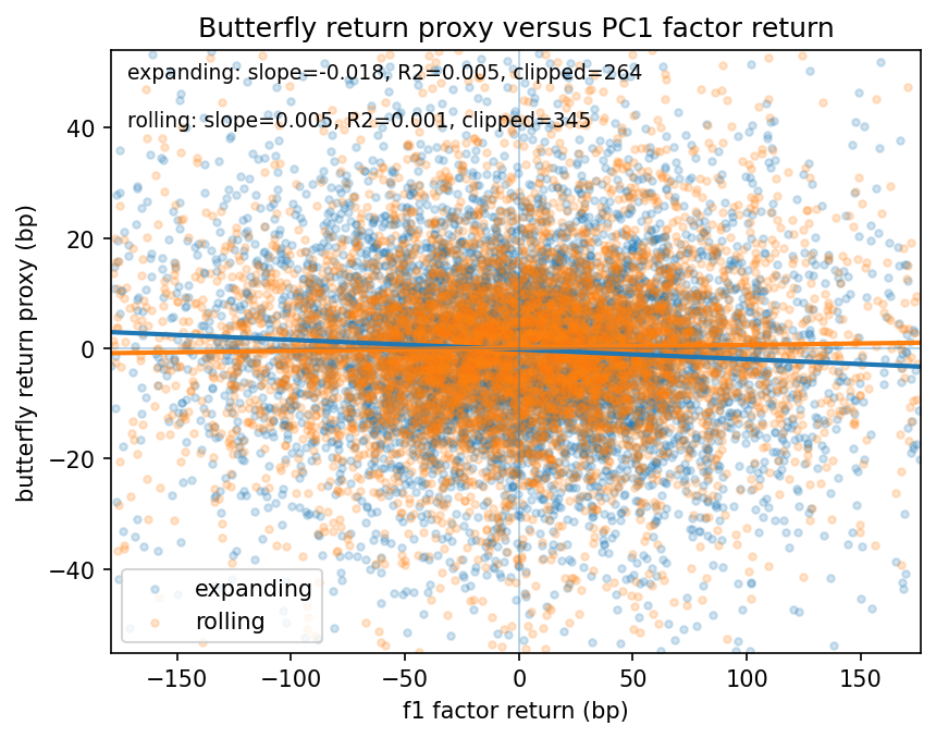
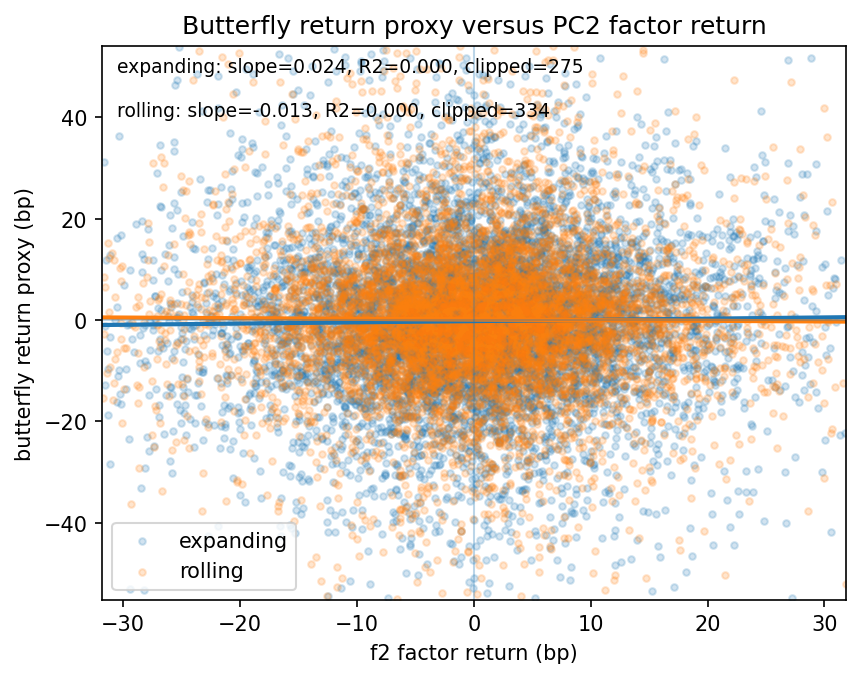
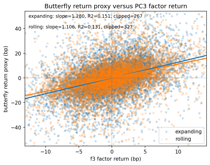
A practical note on why the estimated PC3 exposure can exceed 1 in the realized regression. In theory the three leg hedge is constructed to have unit loading on PC3 and zero loading on PC1 and PC2 at each refit. In practice this mapping is only approximate because the hedge is solved using a three leg restriction while the PCs are estimated on the full curve cross section, and because refit weights are held fixed between refits and then applied to daily factor moves. Small mismatches between the refit basis and the daily factor realization, together with numerical regularization and occasional weight freezing, can lead to a realized PC3 beta that is close to but not exactly 1, and in some samples modestly above 1.

9.3 Performance by era

Because monetary regimes change, I segment performance by era buckets defined during the audit.

Both variants show the strongest performance in the pre 2008 era and negative performance in post 2008 and post 2020. A plausible explanation is that post 2008 policy regimes compressed and distorted curve shape dynamics, weakening mean reversion in residuals designed to target PC3. Another possibility is that the three leg restriction concentrates exposure into higher order factors or microstructure noise when parts of the curve are constrained. These are hypotheses rather than causal claims, and they motivate the tradability extensions in Section 12 and the turnover diagnostics in Section 9.4.

Table 11: Performance by era

Interpretation note: hit_rate here is the daily fraction of positive PnL days within the era (flat days count as non-positive).

variant	series	era	start	end	n_days	ann_ret	ann_vol	sharpe	hit_rate	max_drawdown	avg_turnover	var_95
expanding	gross	pre_2008	1991-01-07 00:00:00	2007-12-31 00:00:00	4250	0.002519	0.024024	0.104872	0.202353	-0.096792	0.093877	-0.002012
expanding	gross	post_2008	2008-01-02 00:00:00	2019-12-31 00:00:00	2995	-0.001744	0.015591	-0.111859	0.196661	-0.053698	0.037964	-0.001466
expanding	gross	post_2020	2020-01-02 00:00:00	2026-01-16 00:00:00	1511	-0.007475	0.010539	-0.709287	0.155526	-0.046974	0.025868	-0.001117
expanding	net	pre_2008	1991-01-07 00:00:00	2007-12-31 00:00:00	4250	0.000154	0.024032	0.006399	0.201412	-0.100461	0.093877	-0.002043
expanding	net	post_2008	2008-01-02 00:00:00	2019-12-31 00:00:00	2995	-0.002701	0.015575	-0.173402	0.196327	-0.054967	0.037964	-0.001466
expanding	net	post_2020	2020-01-02 00:00:00	2026-01-16 00:00:00	1511	-0.008127	0.010569	-0.768896	0.155526	-0.049785	0.025868	-0.001117
rolling	gross	pre_2008	1993-01-12 00:00:00	2007-12-31 00:00:00	3746	0.006417	0.028868	0.222298	0.225841	-0.117342	0.123184	-0.002155
rolling	gross	post_2008	2008-01-02 00:00:00	2019-12-31 00:00:00	2995	-0.005984	0.01258	-0.475704	0.176628	-0.07747	0.038339	-0.00141
rolling	gross	post_2020	2020-01-02 00:00:00	2026-01-16 00:00:00	1511	-0.007427	0.008512	-0.872484	0.147584	-0.050328	0.018561	-0.000756
rolling	net	pre_2008	1993-01-12 00:00:00	2007-12-31 00:00:00	3746	0.003313	0.028865	0.114782	0.224506	-0.120087	0.123184	-0.002157
rolling	net	post_2008	2008-01-02 00:00:00	2019-12-31 00:00:00	2995	-0.00695	0.012578	-0.552584	0.175626	-0.087543	0.038339	-0.001412
rolling	net	post_2020	2020-01-02 00:00:00	2026-01-16 00:00:00	1511	-0.007895	0.008504	-0.928372	0.146923	-0.052754	0.018561	-0.000756

9.4 Turnover and weight distribution

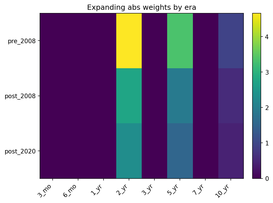
I summarize the distribution of weights and turnover to assess implementation risk. Because the strategy trades a three leg butterfly, the weight heatmap is sparse by design: only the three traded tenors move and all other tenors remain at zero. Extreme refit solves are frozen by design when condition or weight caps trigger, which prevents pathological leverage spikes from unstable solves.

Mean turnover is reported for all days and for active days only (position_state != 0).

Table 12: Turnover summary

variant	mean_turnover_all_days	mean_turnover_active_days	median	p90	max
expanding	0.063016	0.080642	0	0	7.21174
rolling	0.073233	0.096368	0	0	9.74916

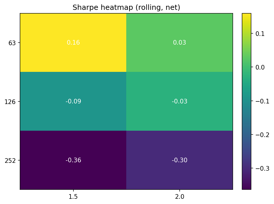
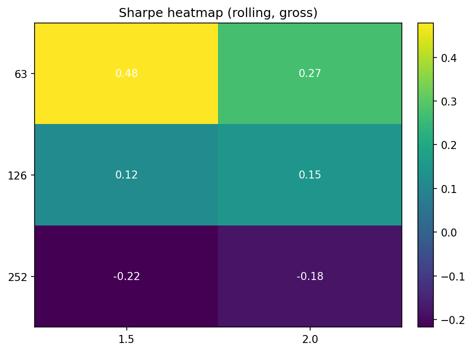
10. Robustness testing

A relative value backtest that only works at one exact setting is often overfit. So I built a robustness grid that reruns the full walk forward pipeline across parameter combinations.

The sweep varies:

1. PCA window length
2. Refit step size
3. Z score window
4. Entry and exit thresholds
5. Expanding versus rolling estimation

Outputs:

1. outputs/section_08/robustness_results.csv
2. outputs/section_08/robustness_heatmap_sharpe_net.png
3. outputs/section_08/robustness_heatmap_sharpe_gross.png

Gross ignores turnover costs; net subtracts linear turnover costs using cost_per_turnover from data/derived/backtest_spec.json (default 1e-4).

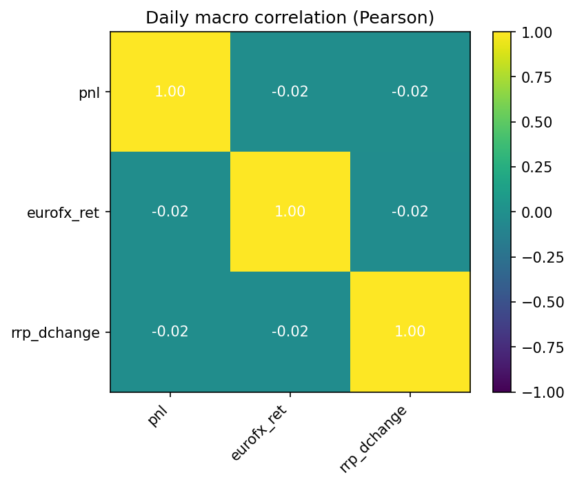
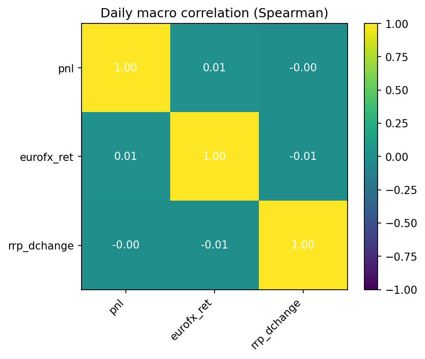
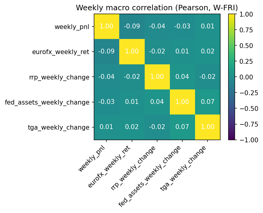
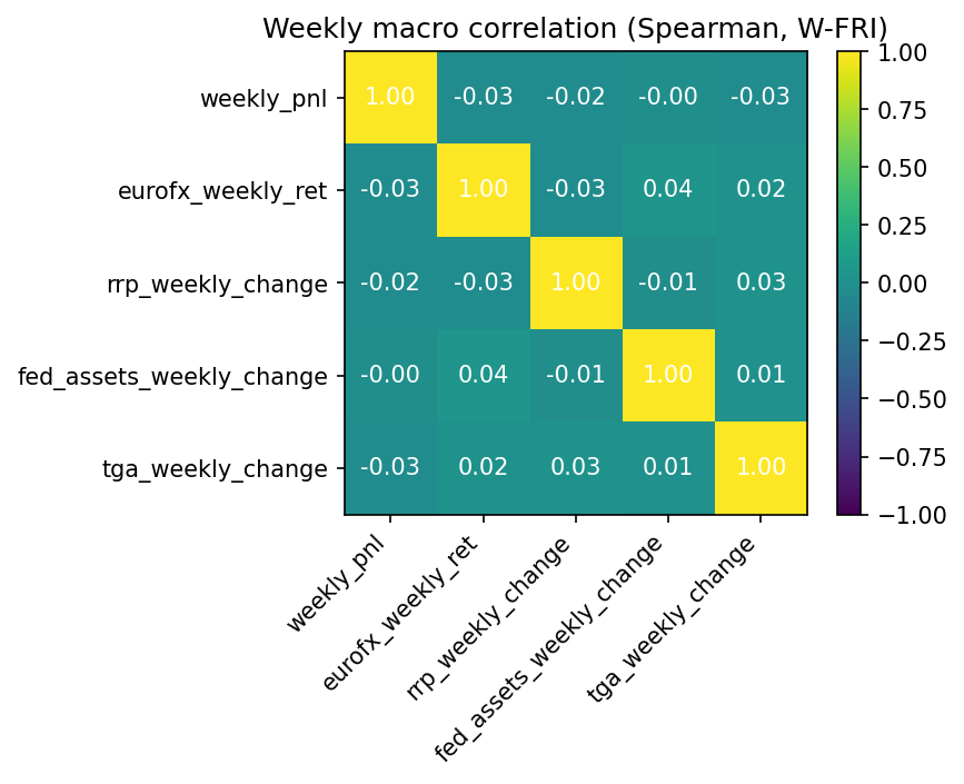
11. Optional macro context checks

As a sanity check, I compute correlations between strategy PnL and macro series at daily and weekly frequency using both Pearson and Spearman measures.

Key output artifacts:

1. outputs/section_08/macro_corr_heatmap_daily_pearson.png
2. outputs/section_08/macro_corr_heatmap_daily_spearman.png
3. outputs/section_08/macro_corr_heatmap_weekly_pearson.png
4. outputs/section_08/macro_corr_heatmap_weekly_spearman.png

Macro correlation heatmaps

12. Limitations and next steps to make it tradeable

Simplifications / non-tradeable assumptions (current notebook)

• Duration proxy uses approximate modified duration from yields under par bond assumptions and is applied with a 1 observation lag in the return proxy.
• Return proxy ignores convexity, carry/roll-down, financing, and funding effects.
• Trading cost uses a linear turnover proxy only.
• Mapping tenor weights to futures/swaps remains future work.

12.1 Instrument mapping

The current strategy constructs weights on curve tenors. A tradeable version would map these exposures to:

1. Treasury futures buckets with duration risk matching and explicit roll rules
2. Swap curve instruments with standardized maturities
3. A hybrid approach that balances liquidity and curve coverage

12.2 Carry, rolldown, and convexity

The duration scaled yield change return proxy isolates first order sensitivity to yield changes. A production model would include:

1. Carry and rolldown per instrument
2. Convexity effects at the long end
3. Financing and margin costs where relevant

12.3 Execution and costs

The cost model is linear in turnover as a placeholder. A realistic model would be instrument specific and include:

1. Bid ask and market impact by instrument and regime
2. Slippage conditional on volatility and liquidity
3. Constraints such as maximum gross duration risk and limits by bucket

12.4 Risk management extensions

The prototype includes max holding and a causality safe signal. Production extensions would add:

1. Volatility targeting or risk parity across regimes
2. Stop logic tied to drawdown or signal breakdown
3. Limits on factor exposure drift

13. Reproducibility and how to navigate the code

This project is written as a coupled notebook and script using a jupytext style structure.

How to run

python -m pip install numpy pandas matplotlib pyarrow tabulate jupytext statsmodels scipy
python rv_project.py

Outputs are written under outputs/section_05, outputs/section_06, outputs/section_07, and outputs/section_08, with intermediate artifacts in data/derived.

Required input data files:

1. data/combined/all_datasets_wide.parquet
2. data/single_assets/treasury_par_yield_curve.parquet

If those files are missing, the script will raise an error during the data load steps.

Main files:

1. rv_project.ipynb
2. rv_project.py

Key derived artifacts:

1. Backtest spec: data/derived/backtest_spec.json
2. Canonical curve: data/derived/curve_treasury_par_canonical.parquet
3. PCA loadings and weights: data/derived/pca_weights_daily_expanding.parquet and related files
4. Residual and z score: data/derived/residual_expanding.parquet, data/derived/zscore_expanding.parquet
5. Backtest outputs: data/derived/bt_daily_expanding.parquet and trade list files
6. Performance outputs: outputs/section_08 (figures and tables)

Figures are written directly into outputs/section_05, outputs/section_06, outputs/section_07, and outputs/section_08.

Suggested reading order in the notebook:

1. Section 2 and Section 3 for data decisions
2. Section 4 for the backtest contract and timing
3. Section 5 for walk forward PCA and the hedging constraints
4. Section 6 and Section 7 for signal construction and trading logic
5. Section 9 and Section 10 for performance and robustness

rv_project.py is canonical and rv_project.ipynb is generated by jupytext sync.

Extra checks

• Refit turnover vs strategy turnover: refit turnover is computed on refit-date weight changes, while strategy turnover is computed on daily position vectors. See outputs/section_08/turnover_refit_vs_strategy.csv plus the component series in outputs/section_05/turnover_refit_rolling.csv and outputs/section_08/turnover_strategy_daily_rolling.csv.
• Rolling flat segments appear driven by repeated freezes rather than missing refits. The long flat stretch in outputs/section_05/rolling_flat_segments.csv shows a high freeze rate (most_common_freeze_reason = weight_cap), and outputs/section_05/refit_schedule_rolling.csv confirms expected refits are present with matching diagnostic rows in outputs/section_05/weight_refit_diagnostics_rolling.csv.